Analytic Solver Data Science provides four options when creating a Neural Network predictor: Boosting & Bagging (ensemble methods), Automatic, and Manual. This example focuses on creating a Neural Network using the boosting ensemble method.
We will use the Boston_Housing.xlsx example data set containing 14 variables described in the table below. The dependent variable MEDV is the median value of a dwelling. The objective of this example is to predict the value of this variable. The CAT. MEDV variable is a categorical variable derived from the MEDV variable, and will not be used in the example.
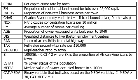
A portion of the data set is shown below.

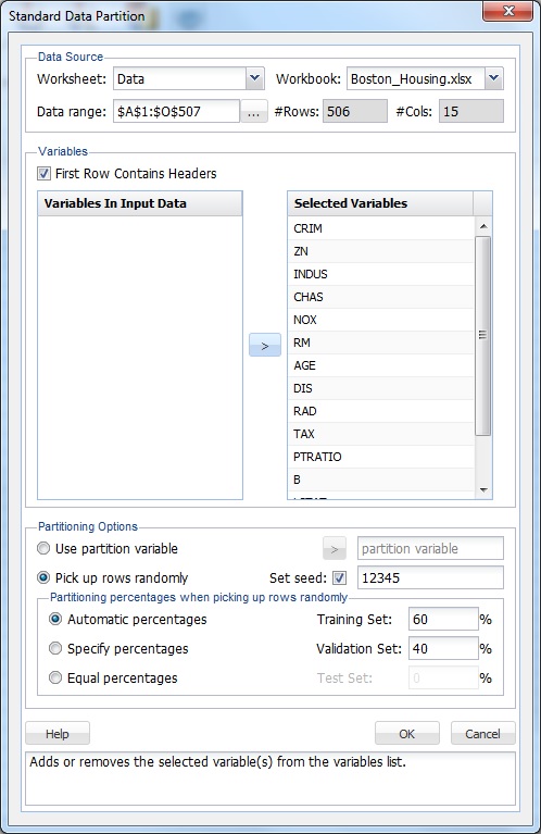
Partition the data into Training and Validation Sets using the Standard Data Partition defaults, with percentages of 60% of the data randomly allocated to the Training Set and 40% of the data randomly allocated to the Validation Set. For more information on partitioning a data set, see the Data Science Partition section.
On the Data Science ribbon, select Partition - Standard Partition to open the Standard Data Partition dialog and select the Boston_Housing workbook.
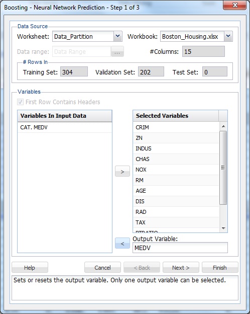
On the Data Science ribbon, select Predict - Neural Network - Boosting to open the Boosting - Neural Network Prediction - Step 1 of 3 dialog.
At Output Variable, select MEDV, then from the Selected Variables list, select all remaining variables (except the CAT.MEDV variable). CAT.MEDV, is a discrete classification of the MEDV variable, and will not be used in this example.
Click Next to advance to the Step 2 of 3 dialog.
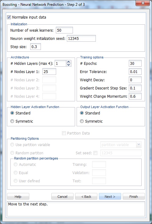
The option Normalize input data is selected by default. Normalizing the data (subtracting the mean and dividing by the standard deviation) is important to ensure that the distance measure accords equal weight to each variable. Without normalization, the variable with the largest scale would dominate the measure.
Leave the Number of weak learners as the default of 50. This option controls the number of weak classification models that will be created. The ensemble method stops when the number or classification models created reaches the value set for the Number of weak learners. The algorithm then computes the weighted sum of votes for each class and assigns the winning classification to each record.
At neuron weight initialization seed, leave the default integer value of 12345. Analytic Solver Data Science uses this value to set the neuron weight random number seed. Setting the random number seed to a non-zero value, ensures that the same sequence of random numbers is used each time the neuron weight are calculated. If left blank, the random number generator is initialized from the system clock, so the sequence of random numbers will be different in each calculation. If you need the results from successive runs of the algorithm to another to be strictly comparable, set the seed.
Internally, the Adaboost algorithm minimizes a loss function using the gradient descent method. The Step size option is used to ensure that the algorithm does not descend too far when moving to the next step. It is recommended to leave this option at the default of 0.3, but any number between 0 and 1 is acceptable. A Step size setting closer to 0 results in the algorithm taking smaller steps to the next point, while a setting closer to 1 results in the algorithm taking larger steps towards the next point.
Keep the default setting of 1 for # Hidden Layers (max 4). Keep the default setting of 25 for # Nodes Per Layer. (Since # hidden layers (max 4) is set to 1, only the first text box is enabled.)
Keep the default setting of 30 for # Epochs. An epoch is one sweep through all records in the Training Set.
Keep the default setting of 0.1 for Gradient Descent Step Size. This is the multiplying factor for the error correction during backpropagation; it is roughly equivalent to the learning rate for the neural network. A low value produces slow but steady learning, a high value produces rapid but erratic learning. Values for the step size typically range from 0.1 to 0.9.
Keep the default setting of 0.6 for Weight change momentum. In each new round of error correction, some memory of the prior correction is retained so that an outlier that crops up does not spoil accumulated learning.
Keep the default setting of 0.01 for Error tolerance. The error in a particular iteration is backpropagated only if it is greater than the error tolerance. Typically, error tolerance is a small value in the range from 0 to 1.
Keep the default setting of 0 for Weight decay. To prevent over-fitting of the network on the training data, set a weight decay to penalize the weight in each iteration. Each calculated weight will be multiplied by (1-decay).
Nodes in the hidden layer receive input from the input layer. The output of the hidden nodes is a weighted sum of the input values. This weighted sum is computed with weights that are initially set at random values. As the network learns, these weights are adjusted. This weighted sum is used to compute the hidden node's output using a transfer function, or activation function. Select Standard (default) to use a logistic function for the activation function with a range of 0 and 1. This function has a squashing effect on very small or very large values but is almost linear in the range where the value of the function is between 0.1 and 0.9. Select Symmetric to use the tanh function for the transfer function, the range being -1 to 1. Keep the default selection of Standard. If more than one hidden layer exists, this function is used for all layers.
As in the hidden layer output calculation, the output layer is also computed using the same transfer function. Select Standard (default) to use a logistic function for the transfer function with a range of 0 and 1. Select Symmetric to use the tanh function for the transfer function, the range being -1 to 1. Select Softmax to use a generalization of the logistic function
Analytic Solver Data Science provides the ability to partition a data set from within a classification or prediction method by selecting Partitioning Options on the Step 2 of 3 dialog. If this option is selected, Analytic Solver Data Science partitions the data set immediately before running the prediction method. If partitioning has already occurred on the data set, this option is disabled. For more information on partitioning, see the Data Science Partition section.
Click Next to advance to the Boosting - Neural Network Prediction - Step 3 of 3 dialog.
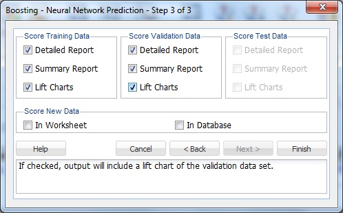
Under Score Training Data and Score Validation Data, Summary Report is selected by default. Under both Score Training Data and Score Validation Data, select Detailed Report, and Lift Charts. Since a Test Data partition was not created, the options under Score Test Data are disabled.
For more information on the Score New Data options, see the Scoring New Data section.
Click Finish to view the output. Click the NNPBoost_Output worksheet to view the Output Navigator.

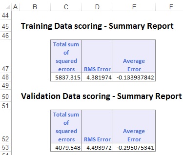
Scroll down until the Summary Reports are displayed for both data sets, and to view how well the Ensemble Method performed. The algorithm finished with an average error of -0.13 in the Training Set and -0.295 in the Validation Set. These small errors indicate that the ensemble method produced a model that is a good fit to the data.
On the Output Navigator, click the NNPBoost_TrainScore tab to view the Prediction of Training Data. Here we see the Predicted Value versus the Actual Value and the Residual for each record in the Training Set.

Click the NNPBoost_ValidScore to view the Prediction of Validation Data. Here we see the Predicted Value versus the Actual Value and the Residual for each record.

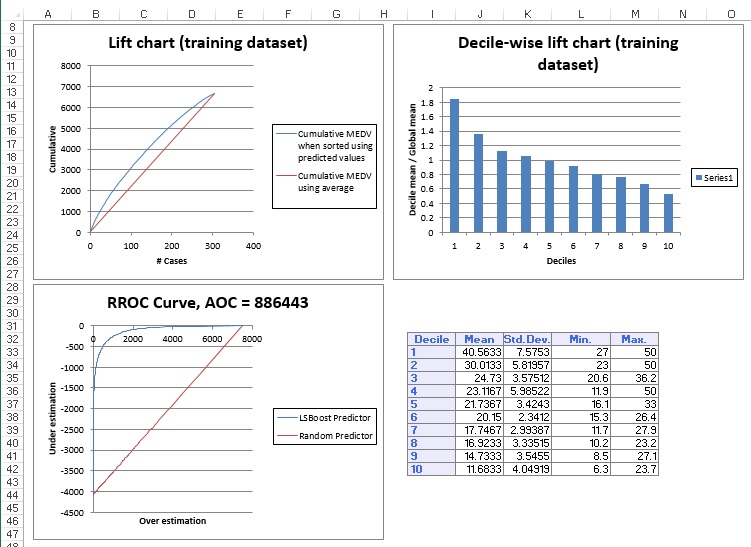
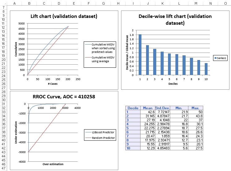
On the Output Navigator, click the NNPBoost_TrainLiftChart and NNPBoost_ValidLiftChart tabs to navigate to the Lift Charts.
Lift charts and RROC Curves are visual aids for measuring model performance. Lift Charts consist of a lift curve and a baseline. The greater the area between the lift curve and the baseline, the better the model. RROC curves plot the performance of regressors by graphing over-estimations (or predicted values that are too high) versus underestimations (or predicted values that are too low.) The closer the curve is to the top left corner of the graph (the smaller the area above the curve), the better the performance of the model.
After the model is built using the Training Set, the model is used to score on theTraining Set and the Validation Set (if one exists). Then the data set(s) are sorted using the predicted output variable value. After sorting, the actual outcome values of the output variable are cumulated and the lift curve is drawn as the number of cases versus the cumulated value. The baseline (red line connecting the origin to the end point of the blue line) is drawn as the number of cases versus the average of actual output variable values multiplied by the number of cases. The decile-wise lift curve is drawn as the decile number versus the cumulative actual output variable value divided by the decile's mean output variable value. This bars in this chart indicate the factor by which the MLR model outperforms a random assignment, one decile at a time. Refer to the validation graph below. In the first decile, taking the most expensive predicted housing prices in the dataset, the predictive performance of the model is a little over 1.8 times better as simply assigning a random predicted value.
In an RROC curve, we can compare the performance of a regressor with that of a random guess (red line) for which under estimations are equal to over estimations shifted to the minimum under estimate. Anything to the left of this line signifies a better prediction, and anything to the right signifies a worse prediction. The best possible prediction performance would be denoted by a point at the top-left of the graph at the intersection of the x and y axis. This point is sometimes referred to as the perfect classification. Area Over the Curve (AOC) is the space in the graph that appears above the ROC curve and is calculated using the formula: sigma2 * n2/2, where n is the number of records The smaller the AOC, the better the performance of the model. In this example we see that the area above the curve in the Training Set is 886,443, and the AOC for the Validation Set is 410,258. Both of these values are rather high. Since the AOC in the RROC curve is related to the variance in the model, we can also take the standard deviation. Doing so, would give us 941.511 ( ) for the Training Set, and 516.416 ( ) for the Validation Set. These values are smaller, but they do still suggest that this model may not be the best fit for this particular data set.
See the Scoring New Data section for information on the Stored Model Sheet, NNC_Stored1.