This example illustrates the random trees ensemble method, the Boston_Housing.xlsx data set and same partition.
On the Analytic Solver Data Science ribbon, select Partition - Standard Partition to open the Standard Partition dialog and select a cell on the Data_Partition worksheet.
On the Analytic Solver Data Science ribbon, select Predict - Regression Tree - Random Trees to open the Regression Tree Random Trees - Step 1 of 3 dialog.
At Output Variable, select MEDV, then from the Selected Variables list, select all remaining variables except CAT.MEDV. (The CAT.MEDV variable is not included in the Input as it is not a categorical variable.)
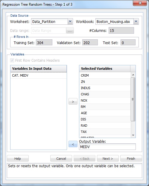
Click Next to advance to the Regression Tree Random Trees- Step 2 of 3 dialog.
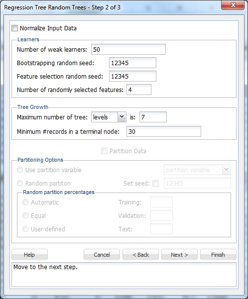
XLMiner normalizes the data when Normalize Input Data is selected. Normalization helps only if linear combinations of the input variables are used when splitting the tree. Keep this option unchecked.
Leave the Number of weak learners at the default of 50. This option controls the number of weak regression models that are created. The ensemble method stops when the number of regression models created reaches the value set for this option.
Leave the default of 12345 for both Bootstrapping random seed and Feature selection random seed. These values set the random seeds during the bootstrap selection portion of the algorithm, or the feature selection portion of the algorithm. Setting a value for these options results in the same observations being chosen for the Training/Validation/Test Sets each time the ensemble method is performed.
The Random Trees ensemble method works by training multiple weak regression trees using a fixed number of randomly selected features, then taking the mode to create a strong regression model. The option Number of randomly selected features controls the fixed number of randomly selected features in the algorithm. Leave this option at the default setting of 4.
Under Tree Growth, leave the defaults of levels and 7 for Maximum number of tree. The tree may also be limited by the number of splits or nodes by clicking the drop-down error next to levels. If levels is chosen, the tree contains the specified number of levels. If splits is selected, the number of times the tree is split is limited to the value entered, and if nodes is selected, the number of nodes in the entire tree will be limited to the value specified.
Keep the default option of 30 for Minimum # records in a terminal node. XLMiner stops splitting the tree when all nodes contain a minimum of 30 records.
XLMiner V2015 provides the ability to partition a data set from within a classification or prediction method by selecting Partitioning Options on the Step 2 of 3 dialog. If this option is selected, XLMiner partitions the data set before running the prediction method. If partitioning has already occurred on the data set, this option is disabled. For more information on partitioning, see the Data Science Partition chapter.
Click Next to advance to the Regression Tree Random Trees - Step 3 of 3 dialog.
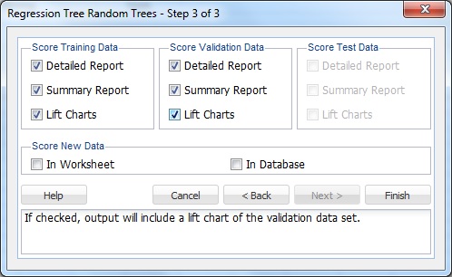
Under both Score Training Data and Score Validation Data, Summary Report is selected by default. Under Score Training Data and Score Validation Data, select Detailed Report and Lift Charts to produce a detailed assessment of the performance of the tree in both sets. Since we did not create a test partition, the options for Score Test Data are disabled. See the Data Science Partition section for information on how to create a test partition.
Click Finish. Worksheets containing the output of the Ensemble Methods algorithm are inserted at the end of the workbook. Click the RTBag_Output worksheet to view the Output Navigator. Click any link to navigate to various sections of the output.

Scroll down the RTRandTrees_Output worksheet to Training Data Scoring - Summary Report to view the Confusion Matrix.
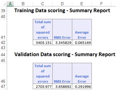
The confusion matrix displays the Total sum of squared errors, the RMS Error, and the Average Error for both data sets. The Average Error for the Training Data is very small at 0.065, and the Average Error for the Validation Data is also small at 0.292. These small error values in both data sets suggest that the Bagging Ensemble Method has created a very accurate predictor. However, these errors are not great measures. RROC curves are much more sophisticated and provide more precise information about the accuracy of the predictor.
Click the RTRandTrees_TrainScore tab to view the Predicted Value, Actual Value, and Residuals for each record in the Training Set.

The same applies to the RTRandTrees_ValidScore tab.

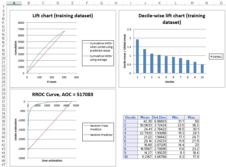
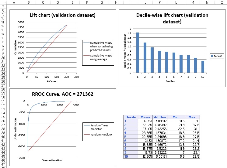
Click the RTRandTrees_TrainLiftChart and RTRandTrees_ValidLiftChart tabs to navigate to the Lift Charts and RROC curves, shown below.
Lift charts and RROC Curves are visual aids for measuring model performance. Lift Charts consist of a lift curve and a baseline. The greater the area between the lift curve and the baseline, the better the model. RROC (regression receiver operating characteristic) curves plot the performance of regressors by graphing over-estimations (or predicted values that are too high) versus under estimations (or predicted values that are too low.) The closer the curve is to the top-left corner of the graph (the smaller the area above the curve), the better the performance of the model.
After the model is built using the Training Set, the model is used to score on the Training Set and the Validation Set (if one exists). Then the data set(s) are sorted using the predicted output variable value. After sorting, the actual outcome values of the output variable are cumulated and the lift curve is drawn as the number of cases versus the cumulated value. The baseline (red line connecting the origin to the end point of the blue line) is drawn as the number of cases versus the average of actual output variable values multiplied by the number of cases. The decile-wise lift curve is drawn as the decile number versus the cumulative actual output variable value divided by the decile's mean output variable value. The bars in this chart indicate the factor by which the MLR model outperforms a random assignment, one decile at a time. Refer to the validation graph below. In the first decile, taking the most expensive predicted housing prices in the data set, the predictive performance of the model is almost two times better as simply assigning a random predicted value.
In an RROC curve, we can compare the performance of a regressor with that of a random guess (red line) for which under estimations are equal to over-estimations shifted to the minimum under estimate. Anything to the left of this line signifies a better prediction and anything to the right signifies a worse prediction. The best possible prediction performance would be denoted by a point at the top left of the graph at the intersection of the x and y axis. This point is sometimes referred to as the perfect classification. Area Over the Curve (AOC) is the space in the graph that appears above the ROC curve and is calculated using the formula: sigma2 * n2/2 where n is the number of records The smaller the AOC, the better the performance of the model. In this example we see that the area above the curve in the Training Set is 517,083 and the AOC for the validation Set is 271,362. Both of these values are rather high. Since the AOC in the RROC curve is related to the variance in the model, we can also take the standard deviation. Doing so would give us 719.08 for the training set and 520.92 for the Validation Set. These values are smaller but they do still suggest that this model may not be the best fit for this particular data set.
Since the number of trees produced when using an Ensemble method can potentially be in the hundreds, it is not practical for XLMiner to draw each tree in the output.
XLMiner generates the RTRandTrees_Stored worksheet along with the other output sheets. For details on scoring data, see the Scoring New Data section.