Time Series Forecasting
Analytic Solver Data Science includes the ability to forecast a future point in a time series in spreadsheet formulas (without using the Score icon on the Applying Your Model tab) using a PsiForecastXxx() function in conjunction with a model created using ARIMA or a smoothing method (Exponential, Double Exponential, Moving Average, or Holt-Winters).
A PsiForecastXxx() function takes as arguments: 1) a table of parameters from a previously-fitted model; and 2) starting values for a new time series, where it is believed that the fitted model is a match for that new time series. When array-entered is used, PsiForecastXxx() returns a forecast of future values for the new time series, for as many periods as there are cells in the array-entry. If the input argument values change, the forecast will be recomputed; but if the input argument values stay the same, and the third argument is FALSE or omitted, the Psi function always returns the same forecast values.
On the Data Science ribbon, from the Applying Your Model tab, select Help - Examples, then select Forecasting/Data Mining Examples to open the Airpass.xlsx example data set. This example data set includes International Airline Passenger Information by month for years 1949-1960. Since the number of airline passengers increases during certain times of the year (i.e., Spring, Summer, and December), this data set includes seasonality.
First, partition the data set into a Training Set and a Validation Set. Use the Training Set to create the ARIMA model, and then apply the model to the Validation Set to forecast six future data points, or one-half year of data.
On the Data Science ribbon, from the Time Series tab, select Partition to open the Time Series Partition Data dialog.
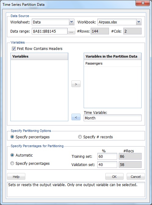
Select Passengers from the Variables in the Partition Data list, and Month for the Time Variable.
Click OK to accept the defaults for Specify Partitioning Options and Specify Percentages for Partitioning. When a time series data set is partitioned, the data set is partitioned sequentially. Therefore, 60% (the first 86 records) are assigned to the Training Set, and the remaining 40% (58 records) are assigned to the Validation Set.
The Data_PartitionTS worksheet is inserted to the right of the Data worksheet. To produce the forecast, on the Data Science ribbon, from the Time Series tab, select ARIMA - ARIMA Model to open the Time Series -ARIMA dialog. Month has been pre-selected as the Time Variable. Select Passengers from the Variables In Input Data list, and click the right arrow to move it to Selected variable.
This example will use a SARIMA model (Seasonal Autoregressive Integrated Moving Average) to predict the next six datapoints in the data set. (For more information on this type of time series model, please see the Exploring a Time Series Data Set section.) A seasonal ARIMA model requires seven parameters, three nonseasonal (autoregressive (p), integrated (d), and moving average (q)), three seasonal (autoregressive (P), integrated (D), and moving average (Q)), and period. Each parameter must be a non-negative integer.
Selecting appropriate values for p, d, q, P, D, Q, and period is beyond the scope of this Help. This example will use a SARIMA model with parameters p = 0, d = 1, q = 1, P = 0, D = 1, Q = 2 and period (P) = 12. For more information on parameter selection, refer to the classic time series analysis text, Time Series Analysis: Forecasting and Control, by George Box and Gwilym Jenkins.
On the Data Science ribbon, from the Time Series tab, select ARIMA - ARIMA Model to open the Time Series - ARIMA dialog. Under ARMA parameters, select Fit seasonal model, and enter 12 for Period (since it takes a full 12 months for the seasonal pattern to repeat). Under Non-seasonal Parameters, set Autoregressive (p) = 0, Difference (d) = 1, and Moving Average (q) = 1. Under Seasonal Parameters, set Autoregressive (P) = 0, Difference (D) = 1, and Moving Average (Q) = 1.
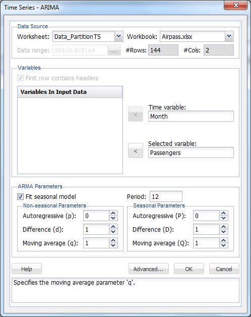
Click OK to create the SARIMA model.
The ARIMA_Output worksheet is inserted to the right of the Data worksheet and contains the Training Error Measures and Fitted Model Statistics. (For more information on this report, see Exploring a Time Series Data Set.) The ARIMA_Stored worksheet is inserted to the right of the Data worksheet and contains the stored model parameters.
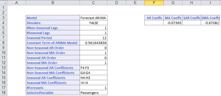
Next, use this ARIMA model to predict new data points in the Validation Set using the PsiForecastARIMA() function. When array-entered into six different Excel cells, this function forecasts six different future points in the data set. (Note: The first forecasted point is more accurate than the second, the second forecasted point more accurate than the third, and so on.) The PsiForecast() function is interactive in the sense that if any of the input values (values passed in the 2nd argument) change, the forecast is recomputed.
The PsiForecastARIMA function takes three arguments: Params, Start_val, and Simulate. Select the Data worksheet and highlight cells B146:B151, then enter =PsiForecastARIMA(.
The first argument, Params, is the range of cells used by Analytic Solver Data Science to store the ARIMA model on the ARIMA_Stored worksheet. This data range changes as the forecast method changes. When entering this first argument, always start with cell B3 and end with the last populated lowest, right-most cell. (There should be no other populated cells to the right or below the last cell in the range.) For this argument, select or enter ARIMA_Stored!B3:I18.
The second argument, Start_val, is the range containing the initial starting points from the Validation data set. The minimum number of initial points that should be specified for a seasonal ARIMA model is the larger of p + d + s * (P + D) and q + s * Q. In this example, p + d + s * (P + D) is equal to 13 (0 + 1 + 12 * (0 + 1) and q + s * Q is equal to 13 (1 + 12 * 1); therefore, the minimum number of initial starting points required is 13 (MAX (13, 13)). If you provide fewer than the minimum required number of starting points, PsiForecastARIMA() will return #VALUE. (See the table below for the minimum number of initial starting points required by each PsiFunctionXxx().) The maximum number of starting points is the number of points in the Validation data set. All points supplied in the second argument will be used in the forecast. For this argument, select or enter Data!B133:B145.
Pass True or False for the third argument. Passing False results in a static forecast that updates if a cell passed in the second argument is changed. If True is passed for this argument, a random error is included in the forecasted points. For this argument, Pass False. See the Time Series Simulation example below for more information on passing True for this argument.
The formula should be the following: =PsiForecastARIMA(ARIMA_Stored!B3:I18,Data!B133:B145, False). Press CTRL+SHIFT+ENTER to enter this formula as an array in all six cells (B146:B151).
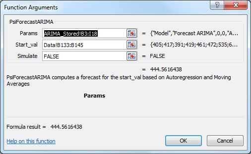
Following are the results from this function.
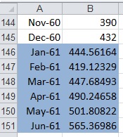
If the any values change in the ranges ARIMA_Stored!B3:I18 or Data!B133:B145, the forecast will be recomputed; but if the input argument values stay the same, the PsiForecastARIMA() function will always return the same forecast values. As mentioned above, the first forecasted value in cell B146 is the most accurate predicted point. Accuracy declines as the number of forecasted points increases.
Time Series Simulation
If your license enables Monte Carlo simulation (i.e., you have Analytic Solver Platform or Analytic Solver Pro is available), V2015 includes the ability to perform a time series simulation, where future points in a time series are forecast on each Monte Carlo trial, using a model created via ARIMA or one of our smoothing methods (Exponential, Double Exponential, Moving Average, or Holt Winters).
To run a time series simulation, True must be passed as the third argument to PsiForecastXxx(), which adds a random (positive or negative) epsilon value to each forecasted point. Each time a simulation is run, 1000 trial epsilon values are generated using the PsiNormal distribution with parameters mean and standard deviation computed by the PsiForecastXxx() function. View the output of this simulation by creating a PsiOutput() function, and then double-clicking the Output cell to view the Simulation Results dialog.
Select cells Data!B146:B151, then from the Excel Formula bar, select Insert Function (fx) to display the Function Argument dialog.
The first argument, ARIMA_Stored!B3:I18, is the range of cells used by Analytic Solver Data Science to store the ARIMA model on the ARIMA_Stored worksheet. This data range changes as the forecast method changes. When entering this first argument, always start with cell B3 and end with the last populated lowest, right-most cell. (There should be no other populated cells to the right or below the last cell in the range.)
For the second argument, the range containing the initial points in the series must be greater than the minimum number of initial points for a static forecast. For a seasonal ARIMA model when Simulate = True, the minimum number of initial points must be greater than Max((p + d + s * (P + D), (q + s * Q). In this example, p + d + s * (P + D) is equal to 13 (0 + 1 + 12 * (0 + 1) and q + s * Q is equal to 13 (1 + 12 * 1); therefore, the minimum number of initial starting points required is 14 (Minimum #Initial Points > MAX (13, 13)). However, when PsiForecastARIMA() is called with Simulate = True, it is recommended to add an additional number of datapoints, equal to the #Periods in the Time Series - ARIMA dialog, to the minimum number required. In this instance the number of initial points will be 25: 13 (minimum # of points) + 12 (# of points for Period in the Time Series - ARIMA dialog). To provide fewer than the minimum required number of starting points (13 in this example), PsiForecastARIMA() will return #VALUE. See the table below for the minimum number of initial starting points required by each PsiFunctionXxx(). All points supplied in the second argument are used in the forecast. Select or enter Data!B132:B145, for this argument.
Passing True for the third argument indicates to Analytic Solver Data Science that this function is used to call in a Monte Carlo simulation, so it should add a random epsilon value (different on each Monte Carlo trial) to each forecasted point.
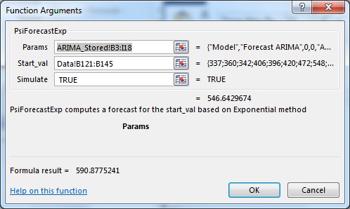
To view the results of the simulation including frequency and sensitivity charts, statistics, and percentiles for the full range of trial values, an output cell must be created. Select cell B146, then from the Excel ribbon, click Analytic Solver Platform. On the ribbon, select the Simulation Model tab, then select Results - Output - Referred Cell. Select cell C146 (or any blank cell on the spreadsheet) to enter the PsiOutput formula. Copy this formula from cell C146 down to cell C151. Therefore, C146 = PsiOutput(B146), C147 = PsiOutput(B147).
On the Analytic Solver Platform ribbon, from the Solve Action tab, select Simulate - Run Once. Analytic Solver Platform performs a simulation with 1,000 Monte Carlo simulation trials (the default number). Since this is the first time a simulation has been performed, the Chart Wizard dialog opens. Subsequent simulations will not produce this report. However, it is possible to re-open the individual frequency charts by double-clicking each of the output cells (B146:B151).
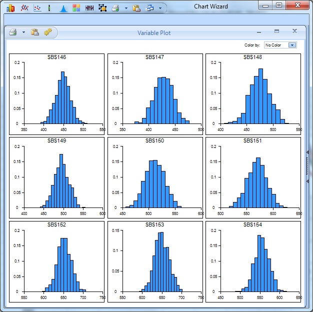
This dialog displays frequency charts for each of the six cells containing the forecasted data points. Double click the chart for cell B146 (top-left) to open the Simulation Results dialog for the PsiForecastARIMA() function in cell B146. From here, you can view frequency and sensitivity charts, statistics, and percentiles for each forecasted point.
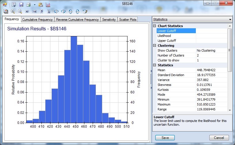
The frequency chart displays the distribution of all 1,000 trial values for cell B146 with an observed mean of 448.79 and standard deviation of 18.92 shown in the Chart Statistics. On the Analytic Solver Platform ribbon, from the Solve Action tab, select Simulate - Run Once (or from the Solver Options and Model Specifications pane, click the green Play button). For each Simulate - Run Once selection, another 1,000 Monte Carlo trials are run, and a different mean is displayed.
In the following dialog, under the Statistics pane, from the Chart Statistics selection, enter 444 for the Lower Cutoff. A vertical bar appears over the Frequency chart to display the frequency with which the forecasted value was greater than this value during the simulation. Use this as an estimate of the probability that the actual value will be less than the forecasted value. In this case, there was a 38.70% chance that the number of international airline passengers would be less than 444,000 in January 1961, and a 61.30% chance that the number of passengers would be greater than 444,000.
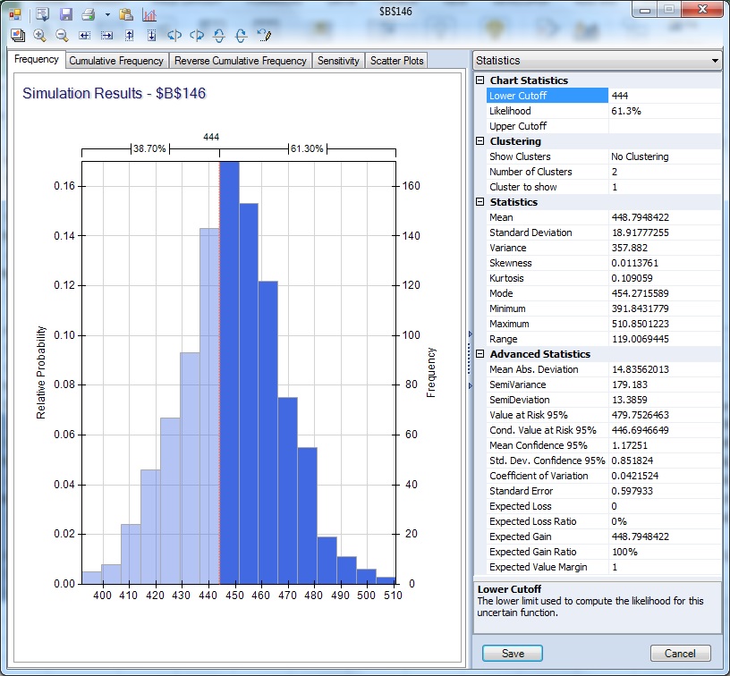
The right column of the Statistics pane includes summary statistics for the full range of forecasted outcomes. The minimum forecasted value during this simulation was 391.84, and the maximum forecasted value was 510.85. In this simulation, the Value at Risk 95% shows that 95% of the time the number of international airline passengers was 479.75, or less in January 1961. The Conditional Value at Risk 95% value indicates that the average number of passengers seen (up to the 95%) was 444.69.
Select cells E146:N146 and then enter the formula, =PsiData(B146), then press CTRL+SHIFT+ENTER to array enter the formula into all 10 cells. Repeat the same steps to array enter “=PsiData(B147)” in cells E147:N147, “=PsiData(B148)” in cells E148:N148, “=PsiData(B149)” in cells E149:N149, “PsiData(B150)” in cells E150:N150, and “=PsiData(B151)” in cells E151:N151. On the Analytic Solver Platform ribbon, from the Solve Action tab, select Simulate - Run Once again to run a simulation.
The ten Excel cells in these columns will update with trial values for each of the PsiForecastARIMA() functions in column B. For example, cells E146:N146 will contain the first 10 trial values for the PsiForecastARIMA() function in cell B146, Cells E147:N147 will contain the first 10 trial values for cell B147, and so on. (For more information on the PsiData() function, see the PSi Function Reference chapter in the Excel Solvers Reference Guide.)
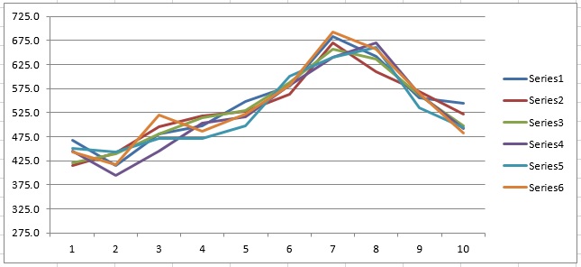
After creating an Excel chart of these values, a chart is displayed (similar to the one below) where each of Series1 through Series6 represents a different Monte Carlo trial. The random epsilon value added to each forecast value accounts for all of the variations among the lines. If the third argument was False or omitted, all of the lines would overlap, assuming that the table or parameters and the starting values were not changing.
The remaining Forecasting methods can be used in the same way using the following information from their respective Stored Model sheets.
Non-Seasonal ARIMA
- Psi Function: PsiForecastARIMA()
- Stored Model Sheet: ARIMA_Stored
- Min # of Initial Points when Simulate = False: Max(p + d, q)
- Min # of Initial points when Simulation = True: Max(p + d, q)
Seasonal ARIMA
- Psi Function: PsiForecastARIMA()
- Stored Model Sheet: ARIMA_Stored
- Min # of Initial Points when Simulate = False: Max(p + d +s * (P + D), q + s * Q)
- Min # of Initial points when Simulation = True: 1 + Max(p + d + s * (P + D), q + s * Q)**
Exponential Smoothing
- Psi Function: PsiForecastExp()
- Stored Model Sheet: Exponential_Stored
- Min # of Initial Points when Simulate = False: 1
- Min # of Initial points when Simulation = True: 1
Double Exponential Smoothing
- Psi Function: PsiForecastDoubleExp()
- Stored Model Sheet: DoubleExponential_Stored
- Min # of Initial Points when Simulate = False: 1
- Min # of Initial points when Simulation = True: 1
Moving Average Smoothing
- Psi Function: PsiForecastMovingAvg()
- Stored Model Sheet: MASmoothing_Stored
- Min # of Initial Points when Simulate = False: # of Intervals
- Min # of Initial points when Simulation = True: # of Intervals
Holt Winters Smoothing
- Psi Function: PsiForecastHoltWinters()
- Stored Model Sheet: HoltWinters_Stored
- Min # of Initial Points when Simulate = False: 2 * #Periods
- Min # of Initial points when Simulation = True: 2 * #Periods
Note: Adding a number of data points equal to the Number of Periods (as shown on the Time Series - ARIMA dialog) to the Minimum # of Initial Points when Simulate = True, is recommended when calling PsiForecastARIMA() with Simulate = True.