VB.NET Product Mix Example
Essential Steps
Follow these steps to define and solve the Product Mix problem in a Visual Basic .NET program (the steps in another Windows programming language would be very similar):
- Create a variable in your program to hold the value of each decision variable in your model.
- Create an assignment statement in your program, that calculates the objective function in your model.
- Similarly, create assignment statements in your program to calculate the left hand sides of your constraints.
- Use SDK objects in your program to tell the Solver about your decision variables, objective and constraint calculations, and desired bounds on constraints and variables.
- Call the Optimize() method in your program to find the optimal solution.
Creating a Visual Basic Program
Assuming that you have Visual Studio and Solver Platform SDK installed, and you've opened a new or existing project, the next step is to define a VB.NET function where the formulas for the objective function and the constraints are calculated.
In the VB.NET code excerpt below, we define a function NLPEvaluator_OnEvaluate() that accesses elements of the model through Solver SDK objects. (Click on the code excerpt for a full-size image.)
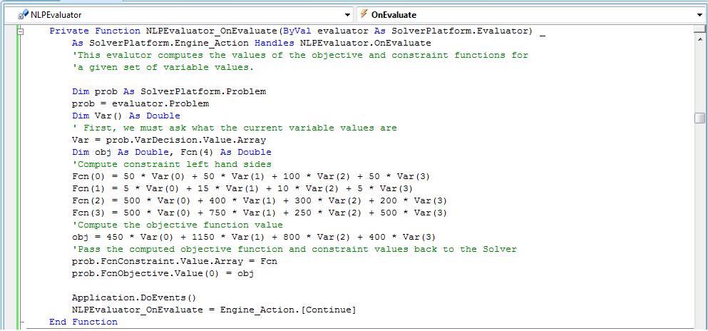
In the above code, we've written the formulas to correspond directly to our earlier outline of the problem (click on Writing the Formulas to see this again). But we could also use Visual Basic arrays and FOR loops to compute these values. (In fact, we can let Solver SDK compute the objective and constraint values for us, using just the coefficients such as 450, 1150, 800 and 400 for the objective function. Read Using the LP Coefficient Matrix Directly in our Advanced Tutorial for more about this option.)
Using the Solver SDK Objects
Next, we must tell the Solver SDK about elements of the model that aren't included in the NLPEvaluator_OnEvaluate() function above. For example, the left hand sides of the constraints are computed in NLPEvaluator_OnEvaluate(), but the constant right hand sides (5800 quarts of glue, 730 hours of pressing capacity, etc.), as well as lower bounds of 0 on the variables, must be specified separately.
To do this, we define an SDK Problem object and set its properties as shown in the code excerpt below. In the last line, we call prob.Solver.Optimize() to find the optimal solution. (Click on the code excerpt for a full-size image.)
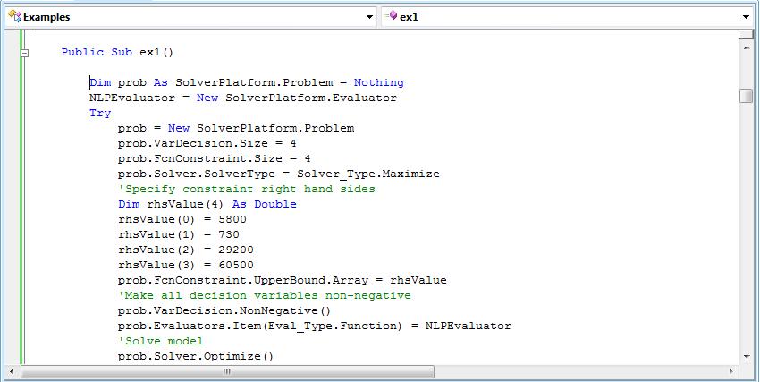
In this code excerpt, FcnUB, FcnLB, VarUB, and VarLB are previously defined arrays, where FcnUB contains the right hand sides of the constraints, and VarLB contains lower bounds of 0 for the variables. Symbolic constants such as Eval_Type.Function, Solver_Type.Maximize, and Problem_Type.OptNLP are predefined in the Solver SDK.
Accessing and Using the Solution
Once the problem is defined and solved, we can use Solver SDK Problem object properties to access the optimal solution. In the code excerpt below, we retrieve the solution status, the objective function value, and the decision variable values at the optimal solution. (Click on the code excerpt for a full-size image.)
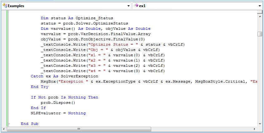
The OptimizeStatus value is an integer code reporting the status of the optimization -- 0 means that an optimal solution was found.
Learning More
If you've gotten to this point, congratulations! You've successfully set up and solved a simple optimization problem using Frontline's Solver Platform SDK. If you'd like, you can see how to set up and solve the same Product Mix problem using Excel's built-in Solver or using Risk Solver Platform in Excel. If you haven't yet read the other parts of the tutorial, you may want to return to the Tutorial Start and read the overviews "What are Solvers Good For?", "How Do I Define a Model?", "What Kind of Solution Can I Expect?" and "What Makes a Model Hard to Solve?"
This was an example of a linear programming problem. Other types of optimization problems may involve quadratic programming, mixed-integer programming, constraint programming, smooth nonlinear optimization, and nonsmooth optimization. To learn more, click Optimization Problem Types. For a more advanced explanation of linearity and sparsity in optimization problems, continue with our Advanced Tutorial.