solver.com

If you'd like to learn more about simulation as well as optimization, consult our tutorials on risk analysis and Monte Carlo simulation.

Derivatives, Gradients, and the Jacobian

Recall the formula we wrote for the objective function in the Product Mix example:

Maximize 75 x1 + 50 x2 + 35 x3 (Profit)

Consider how this function changes as we change each variable x1, x2 and x3.  If we increase x1 by 1, Profit increases by 75; if we decrease x2 by 1, Profit decreases by 50; and so on.  In mathematical terms, 75 is the partial derivative of the objective function with respect to variable x1, and 50 is its partial derivative with respect to x2.

A function of several variables has an overall "rate of change" called its gradient, which is simply a vector of its partial derivatives with respect to each variable:

Similarly, each constraint function has a gradient, which is a vector consisting of the partial derivatives of that function with respect to each decision variable.  The first constraint (Chassis) has a gradient vector [ 1 1 0 ] because it increases by 1 if either x1 or x2 is increased by 1, but it doesn't change if x3 is changed:

1 x1 + 1 x2 + 0 x3 <= 450 (Chassis)
1 x1 + 0 x2 + 0 x3 <= 250 (Picture tubes)
2 x1 + 2 x2 + 1 x3 <= 800 (Speaker cones)
1 x1 + 1 x2 + 0 x3 <= 450 (Power supplies)
2 x1 + 1 x2 + 1 x3 <= 600 (Electronics)

We can combine the gradients of all the constraint functions into a matrix, usually called the Jacobian matrix.  The Jacobian for the Product Mix example looks like this:

Almost every "classical" optimization method, for linear and smooth nonlinear problems, makes use of the objective gradient and the Jacobian matrix of the constraints.

Linearity, Nonlinearity, and Non-Smoothness

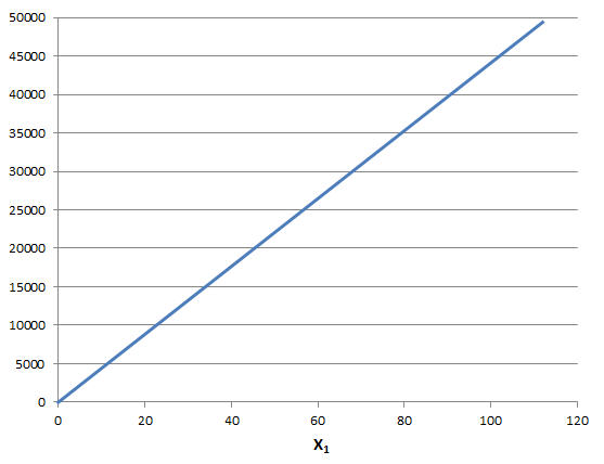
Note that each of these partial derivatives is constant in the Product Mix problem.  For example, the objective function changes by 75 units, whether x1 moves from 0 to 1 or from 100 to 101.  This is true of every linear problem:  In a linear programming problem, the objective gradient and Jacobian matrix elements are all constant.  In this case, the Jacobian matrix (sometimes with the objective gradient as an extra row) is often called the LP coefficient matrix.

Consider a simple nonlinear function such as x1 * x2.  If x1 increases by 1 unit, how much will the function change?  This change is not constant; it depends on the current value of x2.  Even the "square" function x1 * x1 behaves this way.  If, for example, x1 increases from 1 to 2, the function increases from 1 to 4, a change of 3 units.  But if x1 increases from 2 to 3, the function increases from 4 to 9, a change of 5 units.  In a nonlinear optimization problem, the objective gradient and Jacobian matrix elements are not all constant.

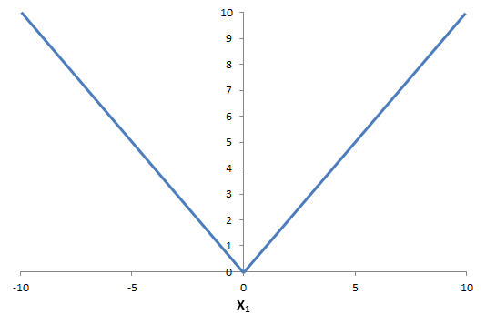
In a smooth nonlinear optimization problem, the partial derivatives may be variable, but they change continuously as the variables change -- they do not "jump" from one value to another.  A nonsmooth function such as ABS(x1) behaves differently:  If x1 is positive, it has a partial derivative of 1, but if x1 is negative, it has a partial derivative of -1.  The partial derivative is discontinuous at 0, jumping between 1and -1.

Mixed Linear and Nonlinear Functions and Terms

Many nonlinear (and even nonsmooth) optimization models include some all-linear constraints and / or some variables that occur linearly in all of the constraints.  Advanced Solvers for smooth nonlinear and nonsmooth problems can gain speed and accuracy by taking advantage of this fact.  The hybrid Evolutionary Solver in the Premium Solver Platform, the Large-Scale GRG Solver engine, and the OptQuest Solver engine are examples of advanced Solvers that work in this way.

Even if a constraint is nonlinear, it may be separated into nonlinear and linear terms.  Similarly, some variables may occur only in the linear terms of otherwise nonlinear constraints.  Some very advanced Solvers -- including a future large-scale nonlinear Solver from Frontline Systems -- are designed to exploit these properties of an optimization problem.

Next:  Using the LP Coefficient Matrix Directly

Back to Tutorial Start