By Francisco Yuraszeck
Using a professional optimization tool like Analytic Solver Upgrade (formerly Premium Solver Pro ) offers multiple benefits that are quickly identified by those starting to learn about the fascinating world of Operations Research.
In my experience as an Operations Research professor, I have personally verified the benefits of computationally implementing optimization models of varying complexity in an intuitive and reliable learning environment. In this sense, students can quickly acquire the necessary skills to deal with different size optimization problems in a platform known, as it turned out.
Furthermore, it is worth noting that Analytic Solver not only allows us to solve optimization models, but also offers the opportunity to create Sensitivity Reports once we have reached the optimal solution and optimal value of the base model. In this context, the sensitivity or post optimal analysis seeks to analyze the impact that a modification of one or several parameters has on the results of a model.
An Analytic Solver Sensitivity Report is divided into 3 parts:
- Objective Cell
- Decision Variable Cells
- Constraints
In the following, we present a simple model of Linear Programming, which will be computationally implemented, giving us the Sensitivity Report that we will then analyze in detail, in order to interpret it in the correct manner.
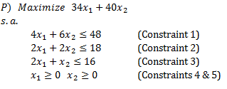
By using Analytic Solver to solve the previous model, we reach the optimal solution X1 = 3 and X2 = 6 , with an optimal value V(LP) = 342 .

In the following, we can obtain the Sensitivity Report by clicking on the module Reports > Optimization > Sensitivity, which will show us the following:

Once we request the Sensitivity Report, a new page will be generated in the Excel file in which we are working, with a report on the results. For the example proposed in this article, we get the following results:

In the following section, we will go over how to interpret each of the three parts that the Sensitivity Report gives us to solve.
- Objective Cell (Max): The optimal value, which is to say, the value reached when evaluating the optimal solution in the objective function, is 342. This value is obtained by: V(P) = 34(3) + 40(6) = 342 .
- Decision Variable Cells: In this section, we can identify the optimal solution (the values in the column labeled Final Value), the coefficients or parameters in the objective function (the values in the Objective Coefficient column), the allowable increase and the allowable decrease for each of the individual coefficients in the objective function, which allows us to guarantee that the current optimal solution is maintained.
For example, let’s consider the coefficient c1 = 34 associated with the variable of decision x1 in the maximization of the objective function. The allowable decrease for said parameter is 7,3 (equivalent to 22/3) units, while the allowable increase is 6, such that if ![]() →
→ ![]() then we maintain the original optimal solution (note that it is assumed that for this analysis, the rest of the model parameters maintain their initial values). Similarly, we recommend that the reader check that the variation interval for keeps the current optimal solution, which is c2ℇ [34,51] .
then we maintain the original optimal solution (note that it is assumed that for this analysis, the rest of the model parameters maintain their initial values). Similarly, we recommend that the reader check that the variation interval for keeps the current optimal solution, which is c2ℇ [34,51] .
It is also interesting to interpret what is known as the Shadow Price of a constraint.
- The Shadow Price corresponds to the exchange rate of the Linear Programming model’s optimal value compared to the marginal modification of the right hand side (RHS) of the constraint. It is understood that a marginal modification allows the conservation of the optimal base of the problem (identical original basic variables in the case of the Simplex Method) or the geometry of the problem (maintain the original active constraints).
Given the previous definition, it is naturally understood that the Shadow Price of Constraint 3 is zero. If the right side represents the availability of a resource (for example, man hours, units of raw material, etc.), 12 of the 16 available units of the resource are used in the original optimal solution (which is consistent with the allowable decrease of 4 units and an allowable increase of 1E+30 or infinity). Additionally, since Constraint 3 is inactive, any variation on the right side of said constraint in the interval ![]() not only conserves the optimal value, but also maintains the optimal original solution.
not only conserves the optimal value, but also maintains the optimal original solution.
The case of Constraints 1 and 2 is different. For example, if Constraint 1 increases on the right side in one unit, moving from 48 to 49 units (note that the allowable increase for said parameter is 6 units), the optimal value will increase proportional to the Shadow Price of said constraint: ![]() . Similarly, if, for example, instead of Constraint 1 increasing on the right side, it falls from 48 to 45 (a drop of 3 units, which is within the permitted range), the new optimal value will be:
. Similarly, if, for example, instead of Constraint 1 increasing on the right side, it falls from 48 to 45 (a drop of 3 units, which is within the permitted range), the new optimal value will be:![]() . We recommend that the reader verify these results him or herself after reoptimizing according to the proposed changes.
. We recommend that the reader verify these results him or herself after reoptimizing according to the proposed changes.
- In summary, it is evident that the usefulness of Analytic Solver lies not only in its ability to implement and computationally solve optimization models. When it comes to correctly interpreting the sensitivity analysis that the program gives us, it allows us to save time by avoiding having to re-optimize many times over. Furthermore, it allows us to better understand the structure of the optimal solution, which is not just limited to identifying values that fit the decision variables in the computational solution.
About the author Francisco Yuraszeck:
University professor in Operational Research and also the owner of the sites www.linearprogramming.info and www.gestiondeoperaciones.net (spanish) which provide in a very simple and educational way the basics and most important topics within this field.