PsiCopula(type, param, [reflection], [instance])
Starting with V2016-R2, Analytic Solver introduces support for Archimedean (and Eliptical) copulas when inducing correlation amongst uncertain variables. Archimedean copula correlation is implemented using the conditional distribution and Laplace-Stieltjes methods.
Type: Analytic Solver supports three types of Archimedean copulas: clayton, frank, and gumbel. The copula type should be passed in quotes as: "clayton", "frank", or "gumbel". In this example, "clayton" is passed. The two elliptical copulas have their own Psi property name: PsiCopulaGauss and PsiCopulaStudent. See below for their signatures.
Param: The parameter of a copula determines the strength of the correlation. In this example, a parameter equal to 10 is passed. See the following parameter restrictions for each Archimedean copula type.
Clayton:
- Bivariate: param >= -1, param ≠ 0.
- Muiltivariate: param > 0
Gumbrel
- Bivariate or Multivariate: param >= 1
Frank
- Bivariate: param ≠ 0.
- Muiltivariate: param > 0
Note: Param = 0 for a multivariate Archimedean copula is supported but indicates no correlation between the uncertain variables.
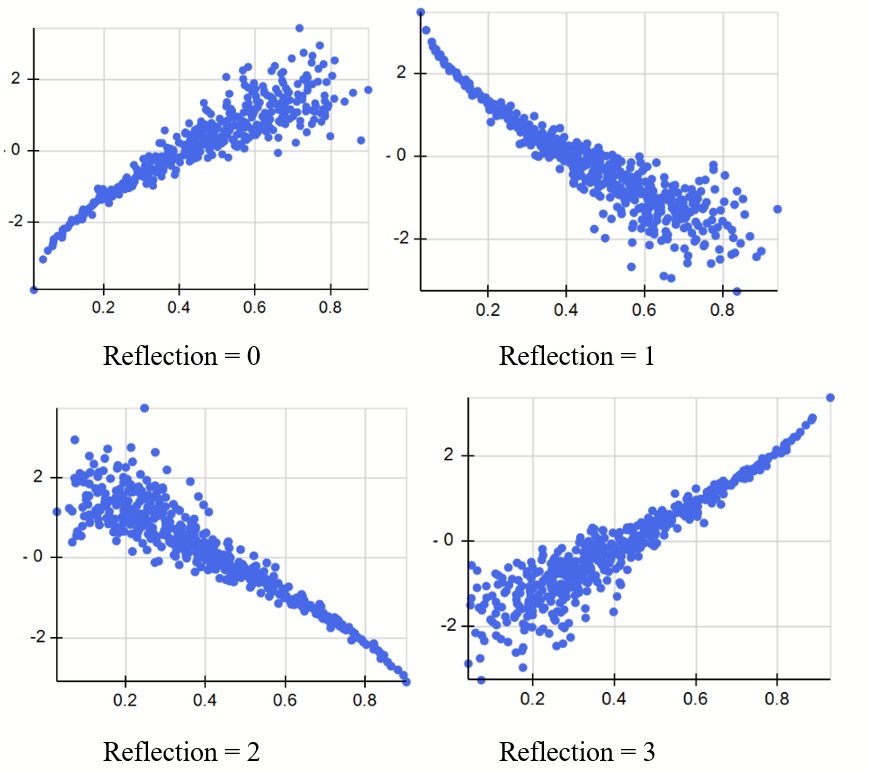
Reflection: (Optional) Analytic Solver allows you to control the direction of a bivariate Archimedean copula using an optional reflection parameter. This argument may take on values of 0, 1, 2, or 3 which controls the reflection of no variables using the value of 0, the 1st variable using the value of 1, the 2nd variable using the value of 2 or both variables using the value of 3. By default, the reflection option is set to 0, which indicates no reflection. In this example, a 0 is passed for the reflection argument to illustrate how this parameter should be passed. In practice, a value of 0 need not be present.
The scatter plots below illustrate the four different positions of a clayton copula correlating two uncertain variables with distributions PsiNormal(0,1) and PsiBeta(3,4).
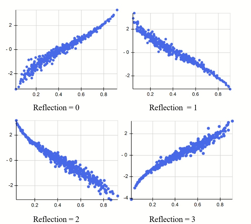
The scatter plots below illustrate the four different positions of a type gumbel copula correlating two uncertain variables with distributions PsiNormal(0,1) and PsiBeta(3,4).
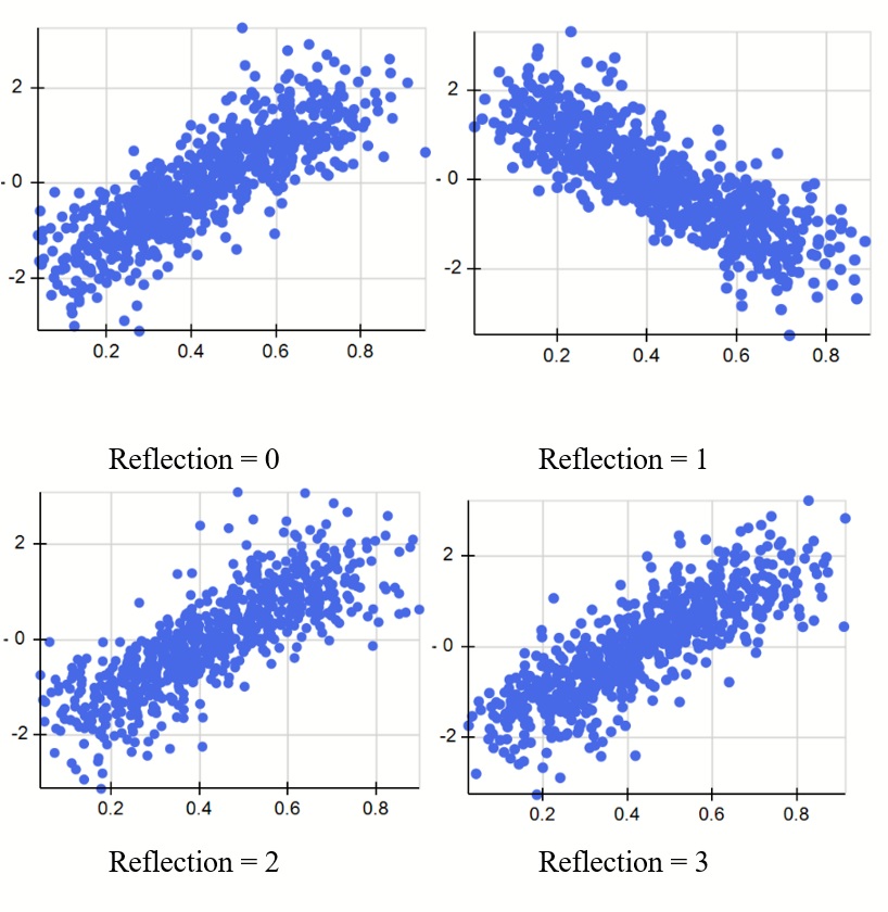
The scatter plots below illustrate the four different positions of a type frank copula correlating two uncertain variables with distributions PsiNormal(0,1) and PsiBeta(3,4). Note: Since the Frank copula is symmetric, this type of copula has only one reflection.
Instance: (Optional) Instance is the string name given to the copula. An Archimedean copula is explicitly identified by the Instance argument and implicitly identified by its argument values. When multiple copulas are present in the same workbook, it is considered "best practice" to use this argument.
Suppose two uncertain variables exist in the same workbook. The PsiCopula property is used to correlate the two uncertain variables using, =PsiCopula("clayton", 10, 0). Since the Instance property is missing, the copula is identified implicitly by its unique set of arguments, in this case ("clayton", "10"). When not passing the Instance property, the PsiCopula property within each uncertain variable signature, MUST use the same arguments. Otherwise, the correlation between the uncertain variables will not be invoked.
Note: PsiCopula("clayton", 10) and PsiCopula("clayton", 10, 0) is considered as the same copula since 0 is the default for the Reflection argument.
To correlate a new group of uncertain variables using a 2nd copula, say PsiCopula("clayton", 12) or PsiCopula("frank", 10), the Instance argument is still not required since either copula is identified by its unique parameters of "clayton" and "12" or "frank" and "10". However, if correlating this same new group of uncertain variables with a copula using the same arguments of "clayton" and "10", a unique name must be passed to the Instance argument, for example, "copula2".
For a complete example of how to use the PsiCopula() property, see the Modeling Correlation Using Copulas section within the Analytic Solver User Guide.
Theory
An Archimedean copula, C, is defined as:
C ( u1, u2, …, um ) = φ-1 ( φ ( u1 ) + … + φ ( ud ; θ ) ; θ )
where φ: [0,1] → [0, ∞) is a strict Archimedean copula generator with inverse φ-1 is completely monotonic on [0, ∞). A strictly decreasing function φ: [0,1]→[0, ∞) that satisfies φ(0) = ∞ and φ(1) = 0. A decreasing function f(t):[a,b]→(-∞, ∞) is completely monotonic if the following equation is satisfied.
-1kdkdtkft≥0,k ϵ N, t ϵa,b
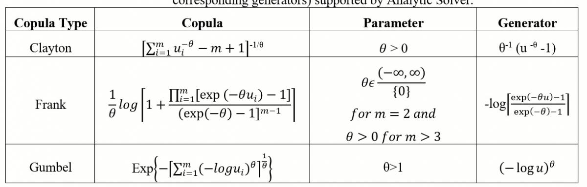
The table below displays the three types of Archimedian copulas, and their corresponding generators) supported by Analytic Solver.
For more information on the theory of Copulas, please see the following references.
Jackel, Peter., “Monte Carlo Methods in Finance”, John Wiley & Sons Ltd, 2002
Nelsen, Roger B., “An Introduction to Copulas”, New York 2006