Optimization requires that we define, in quantitative terms, a model that specifies all the ways, times or places our resources may be allocated, and all the significant constraints on resources and uses that must be met. Here is the way to do that.
Every day, in business, government, and even our personal lives, we make decisions about how to best use the resources – such as time and money – available to us. It is challenging enough for us to decide which items to buy with our available funds, or which of several priorities we should tackle this morning. For even medium-size organizations, this challenge is multiplied many times over: How to best schedule every hour for a staff of 30 people in a call center? How to load packages on a fleet of 100 trucks, and which routes they should drive to make deliveries in the least time? How to assign crews and aircraft to 1,000 airline flights, as they move across the country throughout a day?
These decisions – how to allocate (usually limited) resources to different uses, when there are so many options, with so many interrelationships – are prime candidates for optimization. At leading firms, all the foregoing decisions are routinely made with the aid of optimization. To use optimization, we need to define, in quantitative terms, a model that specifies all the ways, times or places our resources may be allocated, and all the significant constraints on resources and uses that must be met. Then a solver searches for and finds the best resource allocation decisions.
Decision Variables, Objective and Constraints
Our quantified decision variables are the amount of resources allocated to each individual use – for example, the number of call center employees working on each shift, or the number of packages of a given size loaded onto each truck. To determine what “best” means, we must define a quantity called the objective that we can calculate from the values of decision variables—for example, costs that we’d like to minimize or profits to be maximized. To complete the model, we must define each constraint, or limit on the ways resources may be allocated, that reflects the real-world situation. We usually have both simple constraint limits such as “up to 100 trucks,” and constraints calculated from the decision variables, such as “our beginning inventory, plus units received minus units shipped, must equal our ending inventory.”
Let’s consider a very simple example of a call center employee scheduling problem, shown in Figure 1 (this example Excel model is included with Frontline’s Analytic Solver software). Our problem is to schedule enough employees to work each day of the week (decision variables) to handle our predicted call volume (a constraint), while minimizing total payroll cost (our objective).
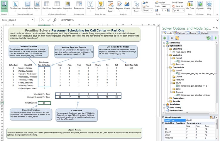
Figure 1: Optimization at work: A Simple Call Center Scheduling Example
Our personnel policy, that employees should work five consecutive days and have two consecutive days off, determines the possible ways that resources can be used: There are seven possible weekly schedules, each one starting on a different day of the week. These are labeled A, B, C through G in the Excel model. For example, employees on Schedule A have Sunday and Monday off, then they work Tuesday through Saturday. Our decision variables – the number of employees working on each schedule – are in cells D15:D21; they are summed in cell D22.
In this simple model, all employees are paid at the same rate, $40 per day at cell N15. Our objective, payroll costs to be minimized, is just =D22*N15*5 (5 working days per week).
We must meet a constraint that the number of employees working each day of the week is greater than or equal to the “Minimum Required Per Day” figures in row 25. We assume here that we actually know these numbers – in many real-world call centers, the call volumes per day are uncertain, and we have only a range or probability distribution for each one. In this tutorial, we’re covering only conventional or deterministic optimization; in a future tutorial, we’ll describe stochastic optimization, where we must allocate resources under conditions of uncertainty in the objective and/or constraints (something that Frontline’s software can handle very well).
The 1s and 0s in the middle of the worksheet help us calculate the number of employees we’ll have in the call center on each day of the week. For example, on Sunday we’ll have the employees on Schedules B through F, but those on Schedules A and G will have the day off. So the number of employees working Sunday is just =SUMPRODUCT(D15:D21,F15:F21) – and similarly for the other days of the week.
Our SUMPRODUCT formulas are in row 24, and we want each value to be greater than or equal to the corresponding “minimum required” number in row 25. We can express this as F24:L24 >= F25:L25, or using Excel defined names, as “Employees per day >= Required per day.” You can see the Solver model taking shape in the right-hand Task Pane in Figure 1.
In this model – as in many others – we must be careful to define all the limits on resources, including “non-negativity.” We cannot have a negative number of employees on any schedule. This may be obvious to us, but Solver does allow negative values for decision variables unless we say otherwise – so we include a constraint D15:D21 >= 0 (or with defined names, “Employees per schedule >= 0”).
There’s one more constraint we haven’t yet discussed: Solver allows any whole number or fractional value for a decision variable, but we can’t actually assign one-half or two-thirds of an employee to a schedule. Indeed, the optimal solution without this integer constraint assigns fractional values to four weekly schedules, such as 2.67 employees for Schedule A, and 6.67 employees for Schedule C – minimizing payroll cost to $4,933.
We complete the Solver model by adding a constraint “Employees per schedule = integer.” (In some optimization software, this is treated as a property of the decision variables, but since it limits the possible solutions, Solver treats these integer requirements as constraints.) We can now solve the model by clicking the Optimize button on the Ribbon, or the green arrow on the Task Pane. The optimal solution ($5,000 payroll cost) is shown in Figure 2: Note that the integer constraint “cost us” something – indeed, additional constraints always yield a “same or worse” objective.
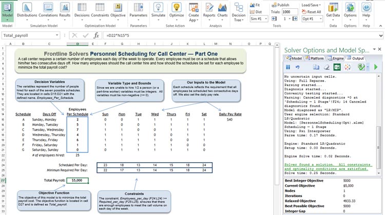
Figure 2: Optimal Solution of the Call Center Scheduling Example
Even more important than the objective value are the decisions that will realize this outcome. These are amounts of resources to be allocated to each use – in this case, the number of employees to be assigned to each of the seven possibly weekly schedules: 2, 5, 7, 4, 6 and 1 for Schedules A, B, C, D, E and F. Because our call volumes on weekends are so high, we assign no employees to Schedule G.
Optimization: Exploiting Structure
How did Solver find this solution, and how do we know that it is the best possible solution? You can play “what-if” with this model, trying different values in cells D15 through D21, searching for a good combination of values. (You’ll find that there is no better combination of values that satisfies all the constraints.) But to really answer this question, we must probe more deeply into “how Solver works,” and talk about some key ideas: optimality conditions, linearity and convexity. Some math and geometry follows(!) – but if you make it all the way through this tutorial, you’ll be rewarded with a much deeper understanding of Solver and optimization.
Solver does try different values for the decision variables, searching for the best solution – indeed all optimization algorithms work this way – but the search is much more sophisticated than randomly chosen “what-if” trials. By computing partial derivatives and testing for satisfaction of the KKT (Karush-Kuhn-Tucker) conditions, Solver can determine that it has found the “top of a peak” or “bottom of a valley” – there are no better solutions “nearby” (a locally optimal solution) – and if the model is convex (discussed later), there are no better solutions anywhere (a globally optimal solution). This yields the message “Solver found a solution. All constraints and optimality conditions are satisfied.”
In our simple Call Center example, Solver had to search a seven-dimensional “space” of possible values for the decision variables (one dimension for each variable), for better objective values, while ensuring that the “Minimum Required” and the non-negativity and integer constraints were satisfied. In a problem with 200 decision variables, this becomes a 200-dimensional search! And Frontline’s enhanced Solvers are routinely used to optimize models with thousands to millions of decision variables.
How? Solver can do this by exploiting the (algebraic) structure of the model. In this case, the objective (recall it is =D22*N15*5, which equals SUM(D15:D21)*40*5) is a linear function of the decision variables. Each of the seven constraints is of the form =SUMPRODUCT(D15:D21, constants), also a linear function of the decision variables. Without the integer constraint, this is a linear programming problem, the easiest type of optimization problem to solve, and one that always yields a globally optimal solution.
When we add the integer constraint, the model becomes a linear mixed-integer programming problem, or LP/MIP as shown in the “Model Diagnosis” area at the bottom of the Task Pane. These problems are significantly harder to solve, but there are sophisticated search algorithms available for LP/MIP problems, and Frontline’s Solvers use them.
Linearity and Convexity: The Keys to Solvability
A linear function, such as SUM or SUMPRODUCT, or any chain of formulas where decision variables are only multiplied by constants and the result added or subtracted, can be plotted as a straight line. In full Analytic Solver software, you can create such a plot (“slicing through” N-dimensional space) with two mouse clicks, Decisions – Plot, as shown for the objective in Figure 3.

Figure 3: Plot of the linear objective function, Total Payroll Cost.
The constraints in our Call Center model also plot as straight lines (in seven-dimensional space). Since they must all be satisfied at the same time, Solver can limit its search to points (i.e., combinations of values for the decision variables) in the intersection of these linear constraints – forming the feasible region. In many dimensions, the intersection of linear constraints is a geometric form called a polytope, but in two dimensions this would be a polygon, as shown (for a different two-variable maximization problem) in Figure 4. The objective – shown in red – is also a straight line that slides up and to the right as it is maximized; the optimal solution is at point D. But the key point is that the polygon or N-dimensional polytope – the feasible region – can be efficiently searched.

Figure 4: Graphical depiction of a two-variable linear programming problem.
From the viewpoint of optimization as a search process, the straight lines in Figure 4 are less important than the overall shape of the feasible region, which is convex. (An intersection of linear constraints is always convex.) A circle, formed by a formula such as x^2 + y^2, is also convex, and is also easy to search; but a non-convex region becomes exponentially harder to search as its dimensionality increases.
Figure 5 shows simple examples of convex and non-convex polygons, in two dimensions. Notice that in the non-convex region, the straight line (called a chord) goes into and out of the feasible region multiple times. A non-convex region has “nooks and crannies,” which take more and more time to search as the dimensionality of the region increases. Imagine, for example, searching a 200-dimensional version of this figure.

Figure 5: Convex and non-convex regions.
When an optimization problem’s objective and constraints are both convex – as is always true in a linear programming problem – the problem will have one optimal solution, which is globally optimal. But a non-convex problem may have many locally optimal solutions.
The Convexity Killers
In Excel models, it is common to use IF functions to make “either-or” choices, and to use CHOOSE or LOOKUP functions to select among multiple values. These functions are very useful, and it’s fine to use them in Solver models, as long as their arguments do not depend on the decision variables.
But if a model has IF, CHOOSE, or LOOKUP functions that do depend on the decision variables, this will quickly make the model both non-convex and non-smooth. Figure 6 shows the type of plot we get for a formula such as =IF(D15<2,F24,3*F24) in our Call Center model.

Figure 6: Plot of IF Function that Depends on Decision Variables.
Compare the “kinks” in this plot to the non-convex region in Figure 5. To make matters worse, the “kinks” make the function non-smooth, which means that Solver cannot reliably compute derivatives at those points – another way of saying that Solver cannot reliably follow the “rate of change” in the function. Again, as the number of dimensions (decision variables) and the number of constraints increases, the time needed to search for an optimal solution increases exponentially.
What can you do, if you need to make “either-or” choices, or select among multiple values in your model? There is a better way: You can express the same conditions using integer variables and linear constraints. Frontline’s Solver User Guide explains how to do this, and our full Analytic Solver software, as part of its model diagnosis, can detect IF, CHOOSE, and LOOKUP functions and automatically replace them with equivalent integer variables and linear constraints, up to a certain level of complexity.
It is worth noting that introducing integer variables into an optimization model actually makes the model non-convex. In Figure 5, because only integer-valued points (which would appear as dots) are feasible, the chords will go “in and out of the feasible region” multiple times. But if integer variables are the only source of non-convexity in the model, then powerful algorithms for handling these integer variables can be applied to greatly cut down on search time. The Gurobi Solver and XPRESS Solver, available as optional plug-in Solver Engines for any of Frontline’s Solver products, are highly effective at solving even large linear mixed-integer and quadratic mixed-integer problems.
Global Optimization
If your model simply cannot be expressed as a linear programming or linear mixed-integer problem, you can still use optimization. In most cases, this means you’ll have to accept an approximate globally optimal solution, a locally optimal solution, or (for a non-convex, non-smooth model) just a “good” solution – better than what you were doing before (this can still yield a great business payoff). Figure 7 is a plot of a smooth but non-convex objective function. You can see that it has multiple “peaks” and “valleys” – the KKT conditions would be satisfied at each peak (when maximizing) or valley (when minimizing), but the globally optimal points are in dark red and dark blue.

Figure 7: A global optimization problem, with just two variables.
Solver in Excel includes basic facilities for global optimization, using either the “Multistart option” for the GRG Nonlinear Solver, or the Evolutionary Solver – and Frontline’s enhanced Solver products offer more powerful methods for global optimization, such as the Interval Global Solver, OptQuest Solver, and Frontline’s hybrid Evolutionary Solver – an engine that combines classical (linear and nonlinear optimization) methods with genetic algorithm, scatter search, local search, and heuristic methods.
If you’ve followed this tutorial to its conclusion, you now know a lot more than most people about optimization! While we’ve illustrated these concepts with Excel models and simple plots, the ideas of linearity and convexity are fundamental, and applicable to any kind of optimization problem, solution algorithm, or software. Hopefully, you also realize how optimization problems can become very difficult to solve, but how powerful software is available to help you find good solutions, even for the most challenging problems.