“Some data analysis tasks cannot be completed in a reasonable time by a human and that makes text mining a useful tool in modern data science and forensics.”
Text mining is the practice of automated analysis of one document or a collection of documents (corpus) to extract non-trivial information. Text mining usually involves the process of transforming unstructured textual data into a structured representation by analyzing the patterns derived from text. The results can be analyzed to discover interesting information, some of which would only be found by a human carefully reading and analyzing the text. Typical, text mining includes but is not limited to Automatic Text Classification/Categorization, Topic Extraction, Concept Extraction, Documents/Terms Clustering, Sentiment Analysis, Frequency-based Analysis and many more.
While you may not deal with datasets in the double-digit millions, using the text mining capabilities of modern analytics software can produce results that can show similar patterns to the data and help you analyze the data more effectively. Here is a brief tutorial on using a major analytics application to develop your text mining capabilities.
Using the Text Miner
Frontline’s Analytic Solver Data Mining's text miner takes an integrated approach to text mining as it does not totally separate analysis of unstructured data from traditional data mining techniques applicable for structured information. While Analytic Solver Data Mining is a very powerful tool for analyzing text only, it also offers automated treatment of mixed data—combinations of multiple unstructured and structured fields. This is a particularly useful feature that has many real-world applications, such as analyzing maintenance reports, evaluation forms, insurance claims, and many other formats.
The text miner uses the “bag of words” model–the simplified representation of text, where the precise grammatical structure of text and exact word order is disregarded. Instead, syntactic, frequency-based information is preserved and is used for text representation. Although such assumptions might be harmful for some specific applications of Natural Language Processing (NLP), it has been proven to work very well for applications such as Text Categorization, Concept Extraction, and other areas addressed by the text miner’s capabilities.
It has been shown in many theoretical/empirical studies that syntactic similarity often implies semantic similarity. One way to access syntactic relationships is to represent text in terms of Generalized Vector Space Model (GVSM). The advantage of such representation is a meaningful mapping of text to the numeric space; the disadvantage is that some semantic elements, such as the order of words, are lost (recall the bag-of-words assumption).
Input to the text miner could be of two main types: a few relatively large documents (for example, several books) or a relatively large number of smaller documents (collection of emails, news articles, product reviews, comments, tweets, Facebook posts). While the text miner can analyze large text documents, it is particularly effective for large corpuses of relatively small documents. Obviously, this functionality has limitless number of applications, for instance, e-mail spam detection, topic extraction in articles, automatic rerouting of correspondence, sentiment analysis of product reviews, and even analyzing net neutrality postings!
The input for text mining is a dataset on a worksheet, with at least one column that contains free-form text—or file paths to documents in a file system containing free-form text—and, optionally, other columns that contain traditional structured data.
The output of text mining is a set of reports that contain general explorative information about the collection of documents and structured representations of text. Free-form text columns are expanded to a set of new columns with numeric representation. The new columns will each correspond to either a single term (word) found in the “corpus” of documents, or, if requested, a concept extracted from the corpus through Latent Semantic Indexing (LSI, also called LSA or Latent Semantic Analysis). Each concept represents an automatically derived complex combination of terms/words that have been identified to be related to a topic in the corpus of documents. The structural representation of text can serve as an input to any traditional data mining techniques available in the text miner: unsupervised/supervised, affinity, visualization techniques, etc.
In addition, the text miner also presents a visual representation of text mining results to allow the user to interactively explore information that would otherwise be extremely hard to analyze manually. Typical visualizations that aid in understanding of Text Mining outputs and that are produced by the text miner are:
- Zipf plot–for visual/interactive exploration of frequency-based information extracted by the text miner
- Scree Plot, Term-Concept and Document-Concept 2D scatter plots–for visual/interactive exploration of Concept Extraction results
If you are interested in visualizing specific parts of text mining analysis outputs, the text miner provides rich capabilities for charting–the functionality that can be used to explore text mining results and supplement the standard charts mentioned.
Here is how to use the text miner to process and analyze approximately 1000 text files and use the results for automatic topic categorization. This will be achieved by using structured representation of text presented to Logistic Regression for building the model for classification. Obviously, it will help your understanding of the process if you have Solver Analytics installed to follow along. The software is available for a trial period at Analytic Solver Data Mining
Getting the data
This example is based on a text dataset that consists of 20,000 messages, collected from 20 different Internet newsgroups. We selected about 1,200 of these messages that were posted to two interest groups, Autos and Electronics (about 500 documents from each). Four folders are created: Autos, Electronics, Additional Autos, and Additional Electronics.
In the text miner, select all files in the folder and the files will appear in the left listbox under Files. Move the files from the Files listbox to the Selected Files listbox. Repeat these steps for the other subfolders. When these steps are completed, 985 files will appear under Selected Files.
Select Sample from selected files to enable the Sampling Options. The text miner will perform sampling from the files in the Selected Files field. Enter 300 for Desired sample size and the text miner will select 300 files using Simple random sampling with a seed value of 12345. Under Output, leave the default setting of Write file paths. Rather than writing out the file contents into the report, the text miner will include the file paths.
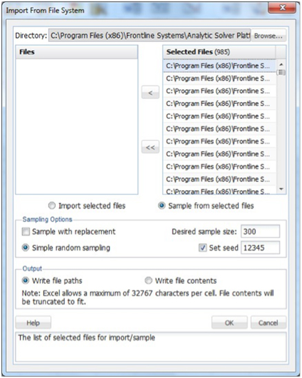
Figure 1
The output XLM_SampleFiles will be inserted into the Data Mining task pane. The Data portion of the report displays the selections made on the Import From File System dialog. Here we see the path of the directories, the number of files written, our choice to write the paths or contents (File Paths), the sampling method, the desired sample size, the actual size of the sample, and the seed value (12345) (Figure 1).
Underneath the Data portion are paths to the 300 text files in random order that were sampled. If Write file contents had been selected, rather than Write file paths, the report would contain the RowID, File Path, and the first 32,767 characters present in the document.
The selected file paths are now in random order, but we will need to categorize the “Autos” and “Electronics” files to be able to identify them later. To do this, we’ll use Excel to sort the rows by the file path. The file paths should now be sorted between Electronics and Autos files.
Confirm that XLM_SampleFiles is selected for Worksheet. Select TextVar in the Variables listbox, and move it to the Selected Text Variables listbox. By doing so, we are selecting the text in the documents as input to the the text miner model. Ensure that “Text variables contain file paths” is checked.
Leave the default setting for Analyze all terms selected under Mode. When this option is selected, the text miner will examine all terms in the document. A “term” is defined as an individual entity in the text, which may or may not be an English word. A term can be a word, number, e-mail, URL, etc. Terms are separated by all possible delimiting characters (i.e. \, ?, ‘, `, ~, |, \r, \n, \t, :, !, @, #, $, %, ^, &, *, (, ), [, ], {, }, <>,_, ;, =, -, +, \) with some exceptions related to stopwords, synonyms, exclusion terms and boilerplate normalization (URLs, e-mails, monetary amounts, etc.). The text miner will not tokenize on these delimiters.
Note: Exceptions are related not to how terms are separated but as to whether they are split based on the delimiter. For example: URL’s contain many characters such as “/” or “;” and the text miner will not tokenize on these characters in the URL but will consider the URL and will remove the URL if selected for removal
If Analyze specified terms only is selected, the Edit Terms button will be enabled. If you click this button, the Edit Exclusive Terms dialog opens. Here you can add and remove terms to be considered for text mining. All other terms will be disregarded. For example, if we wanted to mine each document for a specific part name such as “alternator” we would click Add Term on the Edit Exclusive Terms dialog, then replace “New term” with “alternator” and click Done to return to the Pre-Processing dialog. During the text mining process, the text miner would analyze each document for the term alternator, excluding all other terms.
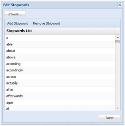
Figure 2
Leave both Start term/phrase and End term/phrase empty under Text Location. If this option is used, text appearing before the first occurrence of the Start Phrase will be disregarded and similarly, text appearing after End Phrase (if used) will be disregarded. For example, if text mining the transcripts from a Live Chat service, you would not be interested in any text appearing before the heading “Chat Transcript” or after the heading “End of Chat Transcript.” You would enter “Chat Transcript” into the Start Phrase field and “End of Chat Transcript” into the End Phrase field (Figure 2).
Leave the default setting for Stopword removal. Click Edit to view a list of commonly used words that will be removed from the documents during pre-processing. To remove a word from the Stopword list, simply highlight the desired word, then click Remove Stopword. To add a new word to the list, click Add Stopword, a new term “stopword” will be added.
The text miner also allows additional stopwords to be added or existing to be removed via a text document (*.txt) by using the Browse button to navigate to the file. Terms in the text document can be separated by a space, a comma, or both. If supplying the three terms in a text document, rather than in the Edit Stopwords dialog, the terms could be listed as: subject emailterm from or subject,emailterm,from or subject, emailterm, from. If we had a large list of additional stopwords, this would be the preferred way to enter the terms.
Advanced in the Term Normalization group allows us to indicate to the text miner, that:
- If stemming reduced term length to 2 or less characters, disregard the term (Minimum stemmed term length).
- HTML tags, and the text enclosed, will be removed entirely. HTML tags and text contained inside these tags often contain technical, computer-generated information that is not typically relevant to the goal of the text mining application.
- URLs will be replaced with the term, “urltoken.” Specific form of URLs do not normally add any meaning, but it is sometimes interesting to know how many URLs are included in a document.
- E-mail addresses will be replaced with the term, “emailtoken.” Since the documents in our collection all contain a great many email addresses (and the distinction between the different e-mails often has little use in text mining), these e-mail addresses will be replaced with the term “emailtoken.”
- Numbers will be replaced with the term, “numbertoken.”
- Monetary amounts will be substituted with “moneytoken.” (Figure 3)
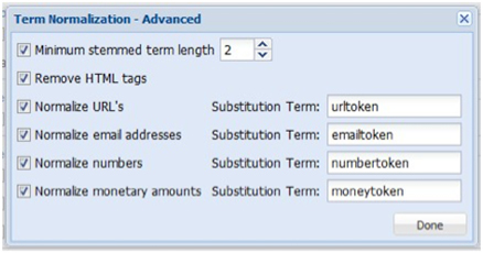
Figure 3
Recall that when we inspected an email from the document collection we saw several terms such as “subject,” “from,” and e-mail addresses. Since all our documents contain these terms, including them in the analysis will not provide any benefit and could bias the analysis. As a result, we will exclude these terms from all documents by selecting Exclusion list then clicking Edit. The label “exclusionterm” is added. Click to edit and change to “subject.” Then repeat these same steps to add the term “from.” We can take the e-mail issue one step further and completely remove the term “emailtoken” from the collection by editing “exclusionterm” to “emailtoken.” We can also enter these terms into a text document (*.txt) and add the terms all at once.
The text miner also allows the combining of synonyms and full phrases by clicking Advanced within Vocabulary Reduction. Select Synonym reduction at the top of the dialog to replace synonyms such as “car,” “automobile,” “convertible,” “vehicle,” “sedan,” “coupe,” “subcompact,” and “jeep” with “auto.” Click Add Synonym and replace “rootterm” with “auto” then replace “synonym list” with “car, automobile, convertible, vehicle, sedan, coupe, subcompact, jeep” (without the quotes) (Figure 4).
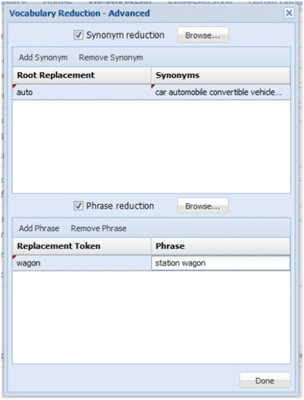
Figure 4
If adding synonyms from a text file, each line must be of the form rootterm:synonymlist or using our example: auto:car automobile convertible vehicle sedan coup or auto:car,automobile,convertible,vehicle,sedan,coup. Note separation between the terms in the synonym list be either a space, a comma or both. If we had a large list of synonyms, this would be the preferred way to enter the terms.
The text miner also allows the combining of words into phrases that indicate a singular meaning such as “station wagon” which refers to a specific type of car rather than two distinct tokens – station and wagon. To add a phrase in the Vocabulary Reduction – Advanced dialog, select Phrase reduction and click Add Phrase. The term “phrasetoken” will appear, click to edit, and enter “wagon.” Click “phrase” to edit and enter “station wagon.” If supplying phrases through a text file (*.txt), each line of the file must be of the form phrasetoken:phrase or using our example, wagon:station wagon.
If you enter 200 for Maximum Vocabulary Size, the text miner will reduce the number of terms in the final vocabulary to the top 200 most frequently occurring in the collection.
Leave Perform stemming as the selected default. Stemming is the practice of stripping words down to their “stems” or “roots.” For example, stemming of terms such as “argue,” “argued,” “argues,” “arguing,” and “argus” would result in the stem “argu.” However, “argument” and “arguments” would stem to “argument.” The stemming algorithm utilized in the text miner is “smart” in the sense that while “running” would be stemmed to “run,” “runner” would not. The text miner uses the Porter Stemmer 2 algorithm for the English Language. For more information on this algorithm, please see: http://tartarus.org/martin/PorterStemmer/
Leave the default selection for Normalize case. When this option is checked, the text miner converts all text to a consistent (lower) case, so that Term, term, TERM, etc. are all normalized to a single token “term” before any processing, rather than creating three independent tokens with different cases. This simple method can dramatically affect the frequency distributions of the corpus, leading to biased results (Figure 5).
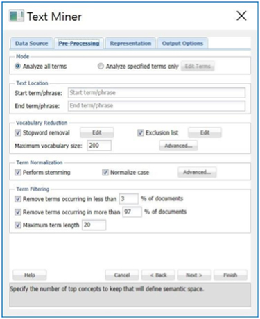
Figure 5
For many text mining applications, the goal is to identify terms that are useful for discriminating between documents. If a term occurs in all or almost all documents, it may not be possible to highlight the differences. If a term occurs in very few documents, it will often indicate great specificity of this term, which is not very useful for some Text Mining purposes. Enter 3 for Remove terms occurring in less than _% of documents and 97 for Remove terms occurring in more than _% of documents.
When you enter 20 for Maximum term length, terms that contain more than 20 characters will be excluded from the text mining analysis and will not be present in the final reports. This option can be extremely useful for removing some parts of text which are not actual English words, for example, URLs or computer-generated tokens, or to exclude very rare terms such as Latin species or disease names, i.e. Pneumonoultramicroscopicsilicovolcanoconiosis.
Keep the default selection of TF-IDF (Term Frequency–Inverse Document Frequency) for Term-Document Matrix Scheme. A term-document matrix is a matrix that displays the frequency-based information of terms occurring in a document or collection of documents. Each column is assigned a term and each row a document. If a term appears in a document, a weight is placed in the corresponding column indicating the term’s importance or contribution.
The text miner offers four different commonly used methods of weighting scheme used to represent each value in the matrix—Presence/Absence, Term Frequency, TF-IDF (the default) and Scaled term frequency. It’s also possible to create your own scheme by selecting choices for local weighting, global weighting, and normalization.
The statistics produced and displayed in the Term-Document Matrix contain basic information on the frequency of terms appearing in the document collection. With this information we can “rank” the significance or importance of these terms relative to the collection and any individual document.
Latent Semantic Indexing, in comparison, uses singular value decomposition (SVD) to map the terms and documents into a common space to find patterns and relationships. For example, if we inspected our document collection, we might find that each time the term “alternator” appeared in an automobile document, the document also included the terms “battery” and “headlights.” Or each time the term “brake” appeared in an automobile document, the terms “pads” and “squeaky” also appeared. However, there is no detectable pattern regarding the use of the terms “alternator” and “brake.” Documents including “alternator” might not include “brake” and documents including “brake” might not include “alternator.” Our four terms—battery, headlights, pads, and squeaky—describe two different automobile repair issues, failing brakes and a bad alternator.
Latent Semantic Indexing will attempt to distinguish between these two different topics, identify the documents that deal with faulty brakes, alternator problems or both, and map the terms into a common semantic space using singular value decomposition. SVD is a tool used by the text miner to extract concepts that explain the main dimensions of meaning of the documents in the collection. The results of LSI are usually hard to examine because the construction of the concept representations will not be fully explained. Interpreting these results is more of an art than a science. However, the text miner provides several visualizations that simplify this process greatly.
Select Maximum number of concepts and increment the counter to 20. Doing so will tell the text miner to retain the top 20 of the most significant concepts. If Automatic is selected, the text miner will calculate the importance of each concept, take the difference between each and report any concepts above the largest difference.
Keep Term frequency table selected (the default) under Preprocessing Summary and select Zipf’s plot. Increase the Most frequent terms to 20 and select Maximum corresponding documents. The Term frequency table will include the top 20 most frequently occurring terms. The first column, Collection Frequency, displays the number of times the term appears in the collection. The second column, Document Frequency, displays the number of documents that include the term. The third column, Top Documents, displays the top 5 documents where the corresponding term appears the most frequently.
The Zipf Plot graphs the document frequency against the term ranks in descending order of frequency. Zipf’s law states that the frequency of terms used in a free-form text drops exponentially, i.e. that people tend to use a relatively small number of words extremely frequently and use a large number of words very rarely.
Th text miner will produce a table displaying the document ID, length of the document, number of terms, and 20 characters of the text of the document. Run the Text Mining analysis and four pop-up charts will appear, and seven output sheets will be inserted into the Model tab of the the text miner task pane.
The Term Count table shows that the original term count in the documents was reduced by 85.54 percent by the removal of stopwords, excluded terms, synonyms, phrase removal and other specified preprocessing procedures. The Documents table lists each Document with its length, number of terms, and if Keep a short excerpt is selected on the Output Options tab and a value is present for Number of characters, then an excerpt from each document will be displayed.
The Term–Document Matrix lists the 200 most frequently appearing terms across the top and the document IDs down the left. If a term appears in a document, a weight is placed in the corresponding column indicating the importance of the term using our selection of TF-IDF on the Representation dialog (Figure 6).
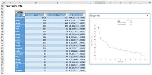
Figure 6
The Final List of Terms table contains the top 20 terms occurring in the document collection, the number of documents that include the term, and the top 5 document IDs where the corresponding term appears most frequently. In this list we would see terms such as “car,” “power,” “engine,” “drive,” and “dealer,” which suggests that many of the documents, even the documents from the electronic newsgroup, were related to autos.
The Zipf Plot shows that our collection of documents follows the power law stated by Zipf. As we move from left to right on the graph, the documents that contain the most frequently appearing terms (when ranked from most frequent to least frequent) drop quite steeply. Hover over each data point to see the detailed information about the term corresponding to this data point.
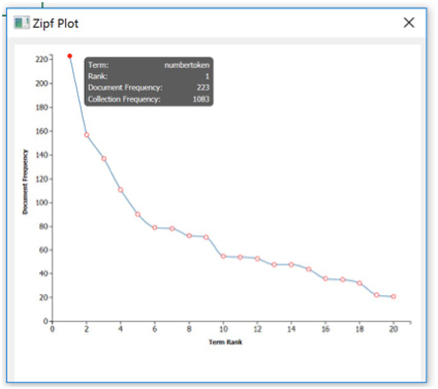
Figure 7
In our exercise, the term “numbertoken” is the most frequently occurring term in the document collection, appearing in 223 documents out of 300 and 1,083 times total. Compare this to a less frequently occurring term such as “thing” which appears in only 64 documents and only 82 times total (Figures 7 & 10).
The Concept Importance table lists each concept, its singular value, the cumulative singular value and the percent singular value explained. The number of concepts extracted is the minimum of the number of documents (985) and the number of terms (limited to 200). These values are used to determine which concepts should be used in the Concept–Document Matrix, Concept–Term Matrix, and the Scree Plot. In this example, we entered “20” for Maximum number of concepts.
The Term Importance table lists the 200 most important terms. To increase the number of terms from 200, enter a larger value for Maximum Vocabulary on the Pre-processing tab of the text miner (Figure 8).
The Scree Plot gives a graphical representation of the contribution or importance of each concept. The largest “drop” or “elbow” in the plot appears between the first and second concept. This suggests that the first top concept explains the leading topic in our collection of documents. Any remaining concepts have significantly reduced importance. However, we can always select more than one concept to increase the accuracy of the analysis. It is best to examine the Concept Importance table and the “Cumulative Singular Value” to identify how many top concepts capture enough information for your application.
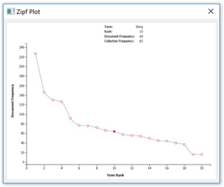
Figure 10
The Concept-Document Scatter Plot is a visual representation of the Concept–Document matrix. Analytic Solver Data Mining normalizes each document representation so it lies on a unit hypersphere. Documents that appear in the middle of the plot, with concept coordinates near 0 are not explained well by either of the shown concepts. The further the magnitude of coordinate from zero, the more effect that concept has for the corresponding document (Figure 11).
In fact, two documents placed at extremes of a concept (one close to -1 and other to +1) indicates strong differentiation between these documents in terms of the extracted concept. This provides means for understanding actual meaning of the concept and investigating which concepts have the largest discriminative power, when used to represent the documents from the text collection.
The Concept–Term Matrix lists the top 20 most important concepts along the top of the matrix and the top 200 most frequently appearing terms down the side of the matrix. The Term-Concept Scatter Plot visually represents the Concept–Term Matrix. It displays all terms from the final vocabulary in terms of two concepts. Similar to the Concept-Document scatter plot, the Concept-Term scatter plot visualizes the distribution of vocabulary terms in the semantic space of meaning extracted with LSA. The coordinates are also normalized, so the range of axes is always [-1,1], where extreme values (close to +/-1) highlight the importance or “load” of each term to a particular concept.
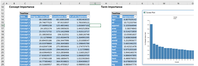
Figure 8
The terms appearing in a zero-neighborhood of concept range do not contribute much to a concept definition. In our example, if we identify a concept having a set of terms that can be divided into two groups, one related to “Autos” and other to “Electronics,” and these groups are distant from each other on the axis corresponding to the concept, this would provide evidence that this particular concept “caught” some pattern in the text collection that is capable of discriminating the topic of article.
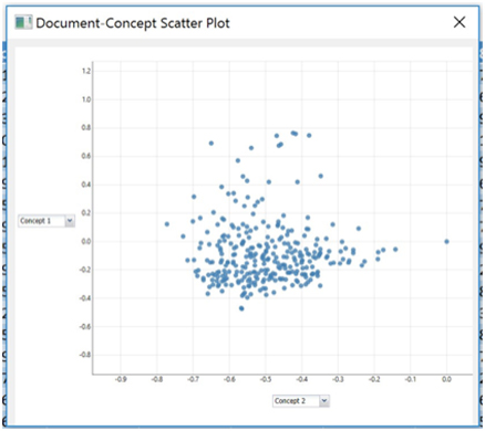
Figure 11
Therefore, Term-Concept scatter plot is an extremely valuable tool for examining and understanding the main topics in the collection of documents, finding similar words that indicate a similar concept, or the terms explaining the concept from “opposite sides”—e.g., term1 can be related to cheap affordable electronics and term2 can be related to expensive luxury electronics.
From here, we can use any of the six classification algorithms to classify our documents according to some term or concept using the Term–Document matrix, Concept–Document matrix, or Concept–Term matrix where each document becomes a “record” and each concept becomes a “variable.”
In this example, we will use the Logistic Regression Classification method to create a classification model using the Concept Document matrix. Recall that this matrix includes the top twenty concepts extracted from the document collection across the top of the matrix and each document in the sample down the left. Each concept will now become a “feature” and each document will now become a “record.”
First, we’ll need to append a new column with the class that the document is currently assigned: electronics or autos. Since we sorted our documents at the beginning of the example starting with Autos, we can simply enter “Autos” into the appropriate column.
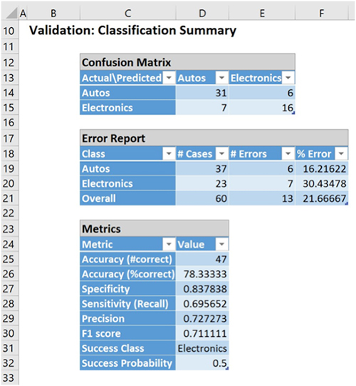
Figure 9
We’ll need to partition our data into two datasets, a training dataset where the model will be “trained,” and a validation dataset where the newly created model can be tested, or validated. When the model is being trained, the actual class label assignments are shown to the algorithm for it to learn which variables (or concepts) result in an “auto” or “electronic” assignment. When the model is being validated or tested, the known classification is only used to evaluate the performance of the algorithm.
Logistic Regression will classify 47 out of a total of 60 documents in the validation partition of our sample, which translates to an overall error of 21.67 percent (Figure 9).
Analytic Solver Data Mining provides powerful tools for importing a collection of documents for comprehensive text preprocessing, quantitation, and concept extraction, to create a model that can be used to process new documents–all performed without any manual intervention. When using the text miner in conjunction with classification algorithms, Analytic Solver Data Mining can be used to classify customer reviews as satisfied/not satisfied, distinguish between which products garnered the least negative reviews, extract the topics of articles, cluster the documents/terms, etc. The applications for text mining are boundless.