
From Optimization: Decision Variables, Objective and Constraints
In many cases, what we really want is the best, or optimal decision under conditions where there is uncertainty and risk. That’s the topic of this tutorial, where we’ll combine ideas from simulation and optimization to build and solve a simulation optimization model.
Our model will have decision variables: amounts of resources allocated to some use or purpose – for example, the number of call center employees working on each shift, or the number of packages of a given size loaded onto each truck. We’ll have an objective such as costs we’d like to minimize, or profits to be maximized, and constraints, or limits on the ways resources may be allocated, that reflects the real-world situation. As we’ll see shortly, dealing with uncertainty means that we must reconsider what it means to maximize or minimize our objective, or to satisfy our constraints.
From Simulation: Uncertain Variables, Distributions and Correlation
Our models will also have uncertain variables. Where decision variables represent quantities that we can control or decide – such as how much to invest, or when to schedule call center employees – uncertain variables represent quantities that we cannot control or decide ourselves – such as stock prices, or the frequency of incoming calls to the call center. To simulate the behavior of uncertain variables, we’ll draw random samples from a probability distribution for each of those variables. In advanced models, we would use rank-order correlation or copulas to deal with the fact that some uncertain quantities are related.
Revisiting a Call Center Scheduling Example
In our fall tutorial on optimization, we used a very simple example of a call center employee scheduling model, shown in Figure 1. Our problem is to schedule enough employees to work each day of the week (decision variables) to handle our predicted call volume (a constraint), while minimizing total payroll cost (our objective).
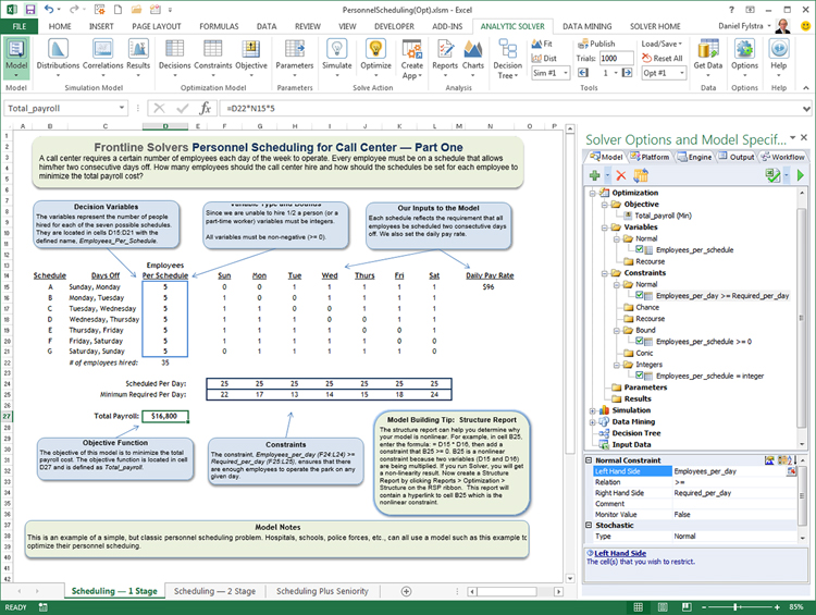
Figure 1: A simple Call Center scheduling example.
Since employees want to work 5 consecutive days and have 2 consecutive days off, there are 7 possible weekly schedules, each one starting on a different day of the week. These are labeled A, B, C through G in the Excel model. For example, employees on Schedule A have Sunday and Monday off, then they work Tuesday through Saturday. Our decision variables – the number of employees working on each schedule – are in cells D15:D21; they are summed in cell D22.
In this simple model, all employees are paid at the same rate, $96 per day at cell N15. So our objective, payroll costs to be minimized, is just =D22*N15*5 (5 working days per week).
In our fall tutorial, we met a constraint that the number of employees working each day of the week is greater than or equal to the “Minimum Required Per Day” figures in row 25. We assumed that we actually knew these numbers – we’ll start there, but in most real-world call centers, the call volumes per day are uncertain, so we’ll tackle that issue later in this tutorial.
The 1s and 0s in the middle of the worksheet help us calculate the number of employees we’ll have in the call center on each day of the week. For example, on Sunday we’ll have the employees on Schedules B through F, but those on Schedules A and G will have the day off. So the number of employees working Sunday is just =SUMPRODUCT(D15:D21,F15:F21) – and similarly for the other days of the week.
Our SUMPRODUCT formulas are in row 24, and we want each value to be greater than or equal to the corresponding “minimum required” number in row 25. We can express this as F24:L24 >= F25:L25, or using Excel defined names, as “Employees_per_day >= Required_per_day”. You can see the Solver model taking shape in the right-hand Task Pane in Figure 1.
We cannot have a negative number of employees on any schedule, so we include a constraint D15:D21 >= 0 (or with defined names, “Employees_per_schedule >= 0”). Solver allows any whole number or fractional value for a decision variable, but we can’t actually assign one-half or two-thirds of an employee to a schedule – so we add a constraint “Employees_per_schedule = integer”.
Solving via Conventional Optimization
We can now solve the model by clicking the Optimize button on the Ribbon, or the “green arrow” on the Task Pane. The optimal solution ($12,000 payroll cost – a big improvement from $18,000 initially) is shown in Figure 2. Solver assigns 2, 5, 7, 4, 6, 1 and 0 employees, respectively, to Schedules A, B, C, D, E, F and G. Since our call volumes are heaviest on weekends, no employees will take both Saturday and Sunday off.
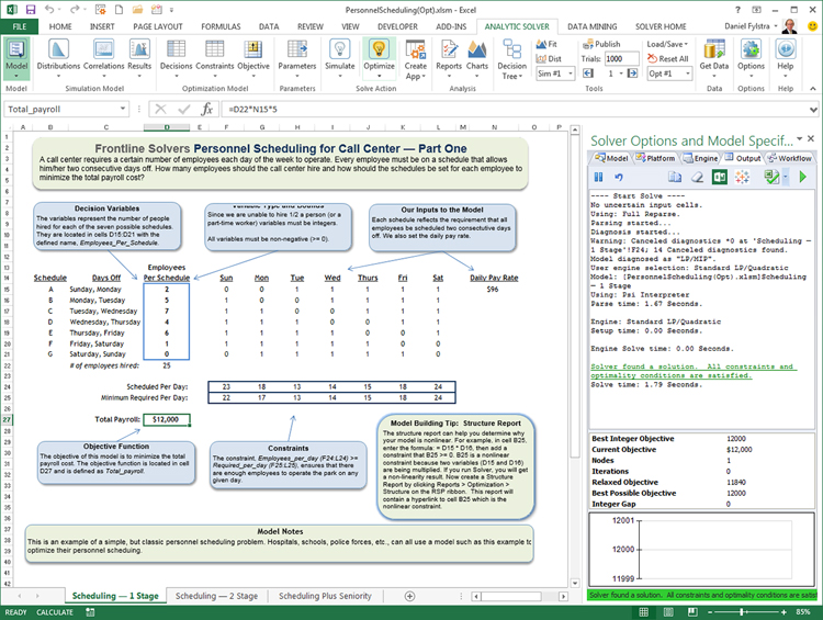
Figure 2: Optimal solution of the Call Center model without uncertainty.
Take a close look at the constraints: Even with the requirement for 5 consecutive working days and 2 consecutive days off, Solver found a way to allocate exactly the minimum required employees on 5 of 7 days; on the other 2 days, just one extra employee was needed. Your intuition might tell you that this is “too tight” – that’s because you can imagine that call volumes, and hence the number of employees needed per day, are not so predictable. But in its current form, the model says that the number needed is known exactly – and Solver is taking full advantage of this.
Far too often in practice, even in large companies and consulting firms, optimization models are built in this way – assuming, implicitly, that the data or parameters of the model are known exactly – which is hardly ever true. If you take nothing else from this tutorial, think about how you can avoid this pitfall! But read on to learn how you can create a better model of a real-world business situation.
Adding Uncertainty to the Model
At present, we have constant numbers in row 25 for the minimum number of employees needed per day: 22 on Sunday, 17 on Monday, 13 on Tuesday, 14 on Wednesday, 15 on Thursday, 18 on Friday, and 24 on Saturday. These are based on the estimated incoming call volume per day, and the average number of calls one employee can handle per day. These quantities are uncertain, not constant: The actual number of calls, and hence the number of employees needed, will fluctuate each day. To keep things simple, we’ll skip the calculations relating call volumes to employees needed, and focus on adjusting the model so the minimum number of employees required per day in row 25 is uncertain.
Drawing from our Monte Carlo simulation tutorial in the summer Solver International, we’ll replace these constant numbers with “generator functions” based on probability distributions. Instead of a fixed number like 22 employees needed on Sunday, we’ll use a LogNormal distribution with a mean value of 22, and a standard deviation of 2. Analytic Solver shows us the “shape” or probability density of this distribution, as shown in Figure 3. Our model now says that we’ll need an uncertain or variable number of employees on Sunday: most (90%) of the time we’ll need between 19 and 25.
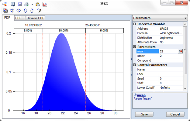
Figure 3: Probability distribution for employees needed on Sunday.
In a similar way, we’ll replace each of the fixed numbers in row 25 with LogNormal distributions, where the mean of the distribution is the same as the fixed number we had before.
To make the model a little more interesting, we’ll add a commission plan for our call center employees. Such a plan would be based on our (uncertain and variable) call volume, but since we’re reflecting that uncertainty in our distributions for the number of employees needed, we’ll just calculate a total commission for the week, based on this number, and add it to our total payroll cost in cell D27. This makes our total payroll cost – which we want to minimize by a smart assignment of employees to schedules – itself an uncertain, variable quantity. Think about that for a minute.
Impact of Uncertainty: Running a Simulation
To see the effect of uncertainty on our model, we can run a Monte Carlo simulation. If you read our Monte Carlo simulation tutorial last summer, you know how this works: Analytic Solver will cause Excel to calculate the model 1,000 or 10,000 times – each such calculation is called a Monte Carlo “trial”. On each trial, Analytic Solver will randomly choose a “sample” value for each of the 7 uncertain variables in row 25, respecting the relative frequencies of the probability distributions – then collect and summarize the results. To do this, we’d better tell Analytic Solver what we want to summarize: The easiest way to do this is to select cell C27 (total payroll cost) and choose Results – Statistics – Mean, “dropping” the result in cell C28.
Starting with our Figure 1 setup, assigning 5 employees to each of the 7 possible schedules, we choose Simulate – Run Once. Analytic Solver displays the simulated results for total payroll cost. Because of our commission plan, this is now a distribution of outcomes, peaking around $18,000, but sometimes less and sometimes more, as shown in Figure 4.
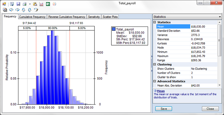
Figure 4: Results from Cell Center model Monte Carlo simulation.
What Does It Mean to Optimize an Uncertain Model?
If you weren’t thinking about this earlier, ask yourself now: What does it mean to “minimize” this wide range of possible values for total payroll cost? We need to tell the software exactly what to do. There is more than one possible answer, but most managers would probably be happy if we can minimize the average (mean) payroll cost, or in the language of probability, the expected value of total payroll cost. Fortunately, in cell C28 we now have an Analytic Solver function =PsiMean(C27) which computes this quantity – so in the next step, we will make C28, not C27, the objective to be minimized in our optimization.
We have a similar issue with our primary constraint “Employees_per_day >= Required_per_day”: For each day of the week, we want the number of employees working that day (in row 24) to cover the minimum number required (in row 25). But those fixed numbers in row 25 are now uncertain variables, representing a wide range of values – as shown in Figure 3. What does it mean to say that a fixed number of employees working on (say) Sunday in F24 is “greater than or equal to” the wide range of values in F25?
We could say that F24 should be greater than the maximum value that is ever sampled for F25 during a simulation – and Analytic Solver would let you do this, for example by placing =PsiMax(F25) in cell F26, and making the constraint F24 >= F26. But that would lead to a high staffing level and payroll cost (a mean of about $20,000, if you try it), and some employees are sure to be idle some of the time. Most managers would say something like “let’s be sure we meet the demand at least 90% of the time” – and Analytic Solver will let you specify this, with =PsiPercentile(F25,90%) in cell F26, and F24 >= F26.
A Simulation Optimization Model
Now that we know what it means to optimize the Call Center model with uncertainty, we can complete the model formulation as shown in Figure 5. Instead of minimizing total payroll cost at C27, we’re minimizing the expected value of total payroll cost across all of our Monte Carlo trials, at C28. Instead of requiring that “Employees_per_day >= Required_per_day”, where “Required_per_day” is now a set of LogNormal distributions, we require that “Employees_per_day >= Required_90th_Percentile”. We still have a lower bound of 0 for each decision variable, but we’ve added an upper bound of 25: This is because Solver Engines suitable for this simulation optimization problem generally require such bounds on the variables, to limit the search space and time.
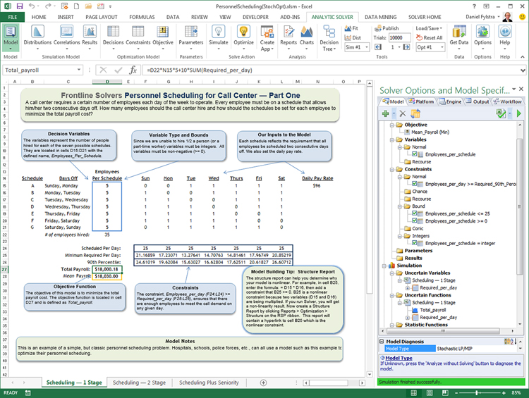
Figure 5: Complete setup of the Cell Center simulation optimization model.
Note that with our original Figure 1 setup, assigning 5 employees to each of the 7 possible schedules, we don’t actually satisfy the constraint “Employees_per_day >= Required_90th_Percentile” on Saturday (and our expected total payroll cost is still about $18,000). The first task for Analytic Solver is to find a feasible solution – one that satisfies all of the constraints.
Solving the Simulation Optimization Model
We’ll use the advanced Evolutionary Solver included as part of Analytic Solver to find a solution, using simulation optimization. The basic idea behind simulation optimization is very simple: An “outer loop” tests different possible values for the decision variables, and within that, an “inner loop” samples many different values for the uncertain variables, computes statistics such as PsiMean() and PsiPercentile(), and returns values that the “outer loop” search process can use.
If you read our fall tutorial on conventional optimization, where we discussed linear programming, linear mixed-integer, nonlinear and global optimization problems, you might wonder what type of problem we’ve created here. Analytic Solver can automatically analyze the algebraic structure of our model: It’s shown in the bottom right of Figure 5, “Stochastic LP/MIP”. This type of model is much harder to solve than a conventional LP/MIP problem, but it’s not the “worst case” of a non-smooth non-convex model.
Figure 6 shows the optimal solution found by the Evolutionary Solver for this model, in about 5 seconds on an average PC. The Evolutionary Solver can use either “genetic algorithm” or “tabu and scatter search” methods – both of these find the same solution, but the genetic algorithm is faster in this case. Unlike our initial setup, we’re now satisfying all of the constraints, and we’ve reduced the expected value of total payroll cost from about $18,000 to $15,150.
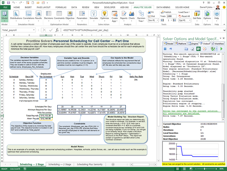
Figure 6: Optimal solution of the Cell Center simulation optimization model.
Conclusion: Welcome to Prescriptive Analytics
In this tutorial, we’ve introduced the approaches you can take to combine Monte Carlo simulation and mathematical optimization methods, to find an optimal solution for the kind of problem that occurs repeatedly in almost every kind of business: allocating scarce resources under conditions of uncertainty.
But we’ve only scratched the surface of what’s possible with modern “prescriptive analytics” tools. There are many more tools available to help formulate models, choose probability distributions or fit them to past data, run multiple, parameterized simulations and optimizations, and much more. And we haven’t even touched upon the topic of stochastic optimization, which aims to find the best decisions for an uncertain future. So we hope you’ll stayed tuned for more insights about real-world prescriptive analytics, in future issues of Solver International.