This example focuses on creating a Neural Network using an Automated network architecture. See the section below for an example on creating a Neural Network using a Manual Architecture.
Click Help – Example Models on the Data Science ribbon, then click Forecasting/Data Science Examples to open the file Wine.xlsx.
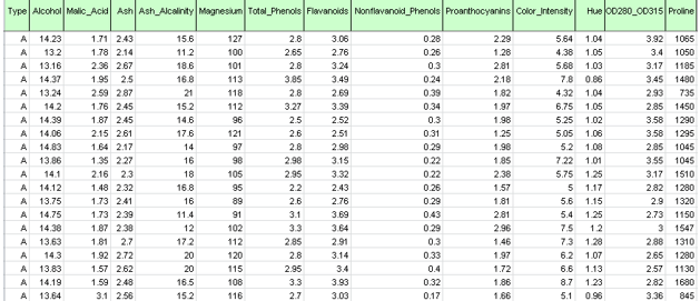
This file contains 13 quantitative variables measuring the chemical attributes of wine samples from 3 different wineries (Type variable). The objective is to assign a wine classification to each record. A portion of this dataset is shown below.
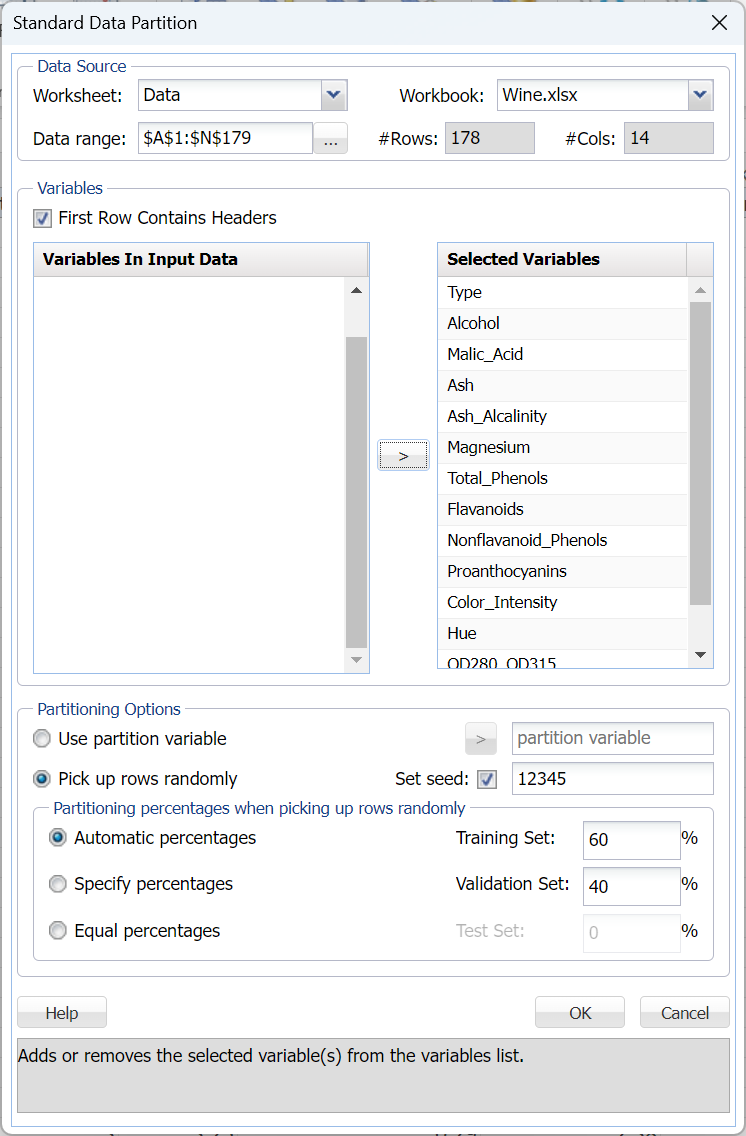
First, we partition the data into training and validation sets using a Standard Data Partition with percentages of 60% of the data randomly allocated to the Training Set and 40% of the data randomly allocated to the Validation Set. For more information on partitioning a dataset, see the Data Science Partitioning chapter.
Click Next to advance to the next tab.
When an automated network is created, several networks are run with increasing complexity in the architecture. The networks are limited to 2 hidden layers and the number of hidden neurons in each layer is bounded by UB1 = (#features + #classes) * 2/3 on the 1st layer and UB2 = (UB1 + #classes) * 2/3 on the 2nd layer.
First, all networks are trained with 1 hidden layer with the number of nodes not exceeding the UB1 and UB2 bounds, then a second layer is added and a 2 – layer architecture is tried until the UB2 limit is satisfied.
The limit on the total number of trained networks is the minimum of 100 and (UB1 * (1+UB2)). In this dataset, there are 13 features in the model and 3 classes in the Type output variable giving the following bounds:
UB1 = FLOOR(13 + 3) * 2/3 = 10.67 ~ 10
UB2 = FLOOR(10 + 3) * 2/3 = 8.67 ~ 8
(where FLOOR rounds a number down to the nearest multiple of significance.)
# Networks Trained = MIN {100, (10 * (1 + 8)} = 90
As discussed in previous sections, Analytic Solver Data Science includes the ability to partition a dataset from within a classification or prediction method by clicking Partition Data on the Parameters tab. If this option is selected, Analytic Solver Data Science will partition your dataset (according to the partition options you set) immediately before running the classification method. If partitioning has already occurred on the dataset, this option will be disabled. For more information on partitioning, please see the Data Science Partitioning chapter.
Click Rescale Data to open the Rescaling dialog. Use Rescaling to normalize one or more features in your data during the data preprocessing stage. Analytic Solver Data Science provides the following methods for feature scaling: Standardization, Normalization, Adjusted Normalization and Unit Norm. For more information on this new feature, see the Rescale Continuous Data section within the Transform Continuous Data chapter that occurs earlier in this guide.
For this example, select Rescale Data and then select Normalization. Click Done to close the dialog.
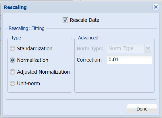
Note: When selecting a rescaling technique, it's recommended that you apply Normalization ([0,1)] if Sigmoid is selected for Hidden Layer Activation and Adjusted Normalization ([-1,1]) if Hyperbolic Tangent is selected for Hidden Layer Activation. This applies to both classification and regression. Since we will be using Logistic Sigmoid for Hidden Layer Activation, Normalization was selected.
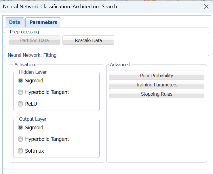
Click Prior Probability. Three options appear in the Prior Probability Dialog: Empirical, Uniform and Manual.
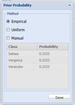
If the first option is selected, Empirical, Analytic Solver Data Science will assume that the probability of encountering a particular class in the dataset is the same as the frequency with which it occurs in the training data.
If the second option is selected, Uniform, Analytic Solver Data Science will assume that all classes occur with equal probability.
Select the third option, Manual, to manually enter the desired class and probability value.
Click Done to close the dialog and accept the default setting, Empirical.
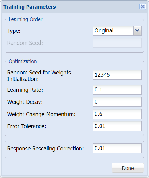
Users can change both the Training Parameters and Stopping Rules for the Neural Network. Click Training Parameters to open the Training Parameters dialog. For more information on these options, please see the Neural Network Classification Options section below. For now, simply click Done to accept the option defaults and close the dialog.
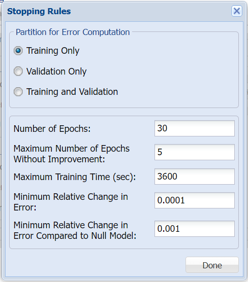
Click Stopping Rules to open the Stopping Rules dialog. Here users can specify a comprehensive set of rules for stopping the algorithm early plus cross-validation on the training error. For more information on these options, please see the Neural Network Classification Options section below. For now, simply click Done to accept the option defaults and close the dialog.
Keep the default selections for the Hidden Layer and Output Layer options. See the Neural Network Classification Options section below for more information on these options.
Click Finish. Output sheets are inserted to the right of the STDPartition worksheet.
NNC_Output
Click NNC_Output to open the first output sheet.
The top section of the output includes the Output Navigator which can be used to quickly navigate to various sections of the output. The Data, Variables, and Parameters/Options sections of the output all reflect inputs chosen by the user.
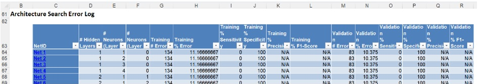
A little further down is the Architecture Search Error Log, a portion is shown below.
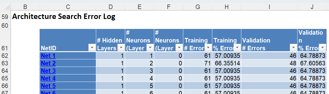
Notice the number of networks trained and reported in the Error Report was 90 (# Networks Trained = MIN {100, (10 * (1 + 8)} = 90).
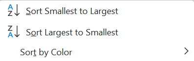
This report may be sorted by each column by clicking the arrow next to each column heading. Click the arrow next to Validation % Error and select Sort Smallest to Largest from the menu. Then click the arrow next to Training % Error and do the same to display all networks 0% Error in both the Training and Validation sets.
Click a Net ID, say Net 2, hyperlink to bring up the Neural Network Classification dialog. Click Finish to run the Neural Net Classification method with Manual Architecture using the input and option settings specified for Net 2.
The layout of this report changes when the number of classes is reduced to two. Please see the section NNC with Output Variable Containing 2 Classes below for an example with a dataset that includes just two classes.
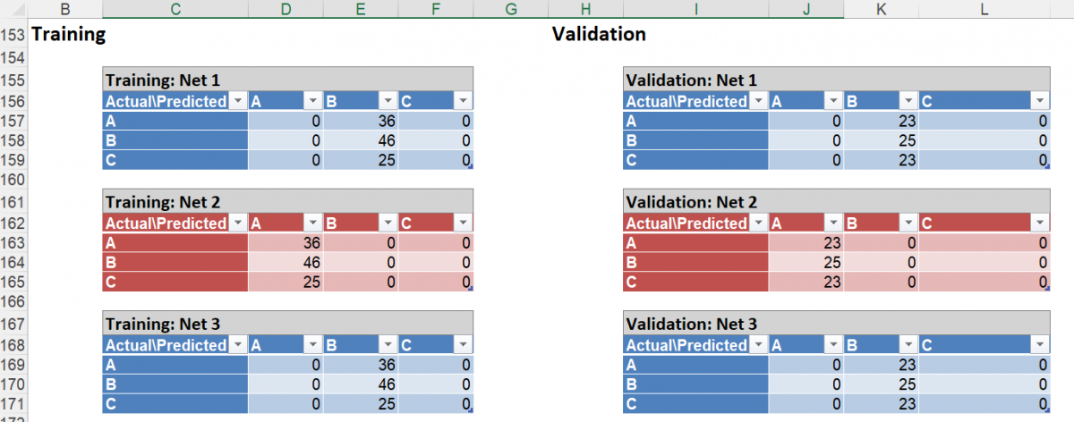
Scroll down on the NNC_Output sheet to see the confusion matrices for each Neural Network listed in the table above. Here’s the confusion matrices for Net 1and 2. These matrices expand upon the information shown in the Error Report for each network ID.
Output Variable Containing Two Classes
The layout of this report changes when the number of classes is reduced to two. See the example report below.
The Error Report provides the total number of errors in the classification -- % Error, % Sensitivity or positive rate, and % Specificity or negative rate -- produced by each network ID for the Training and Validation Sets. This report may be sorted by column by clicking the arrow next to each column heading.
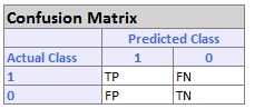
Sensitivity and Specificity measures are unique to the Error Report when the Output Variable contains only two categories. Typically, these two categories can be labeled as success and failure, where one of them is more important than the other (i.e., the success of a tumor being cancerous or benign.) Sensitivity (true positive rate) measures the percentage of actual positives that are correctly identified as positive (i.e., the proportion of people with cancer who are correctly identified as having cancer). Specificity (true negative rate) measures the percentage of failures correctly identified as failures (i.e., the proportion of people with no cancer being categorized as not having cancer). The two are calculated as in the following (displayed in the Confusion Matrix).
Sensitivity or True Positive Rate (TPR) = TP/(TP + FN)
Specificity (SPC) or True Negative Rate =TN / (FP + TN)
If we consider1 as a success, the Confusion Matrix would appear as in the following.
When viewing the Net ID 10, this network has one hidden layer containing 10 nodes. For this neural network, the percentage of errors in the Training Set is 3.95%, and the percentage of errors in the Validation Set is 5.45%.The percent sensitivity is 87.25 % and 89.19% for the training partition and validation partition, respectively. This means that in the Training Set, 87.25% of the records classified as positive were in fact positive, and 89.19% of the records in the Validation Set classified as positive were in fact positive.
Sensitivity and Specificity measures can vary in importance depending upon the application and goals of the application. The values for sensitivity and specificity are pretty low in this network, which could indicate that alternate parameters, a different architecture, or a different model might be in order. Declaring a tumor cancerous when it is benign could result in many unnecessary expensive and invasive tests and treatments. However, in a model where a success does not indicate a potentially fatal disease, this measure might not be viewed as important.
The percentage specificity is 87.23% for the Training Set, and 95.76% in the Validation Set. This means that 87.23% of the records in the training Set and 95.76% of the records in the Validation Set identified as negative, were in fact negative. In the case of a cancer diagnosis, we would prefer that this percentage be higher, or much closer to 100%, as it could potentially be fatal if a person with cancer was diagnosed as not having cancer.