This example focuses on creating a Neural Network using the Automatic Architecture. See the Ensemble Methods chapter that appears later on in this guide to see an example on creating a Neural Network using the boosting and bagging ensemble methods. See the section below for an example of how to create a single neural network.
We will use the Boston_Housing.xlsx example dataset. This dataset contains 14 variables, the description of each is given in the Description worksheet. The dependent variable MEDV is the median value of a dwelling. This objective of this example is to predict the value of this variable.
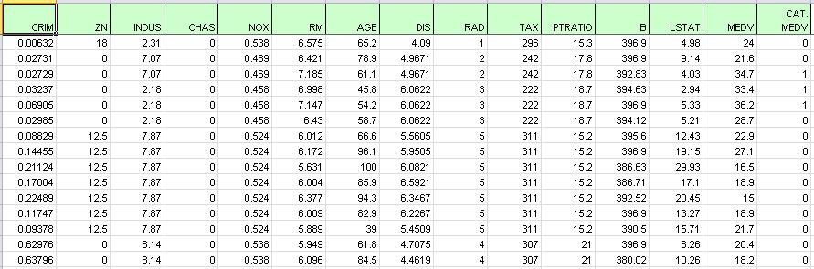
A portion of the dataset is shown below. The last variable, CAT.MEDV, is a discrete classification of the MEDV variable and will not be used in this example.
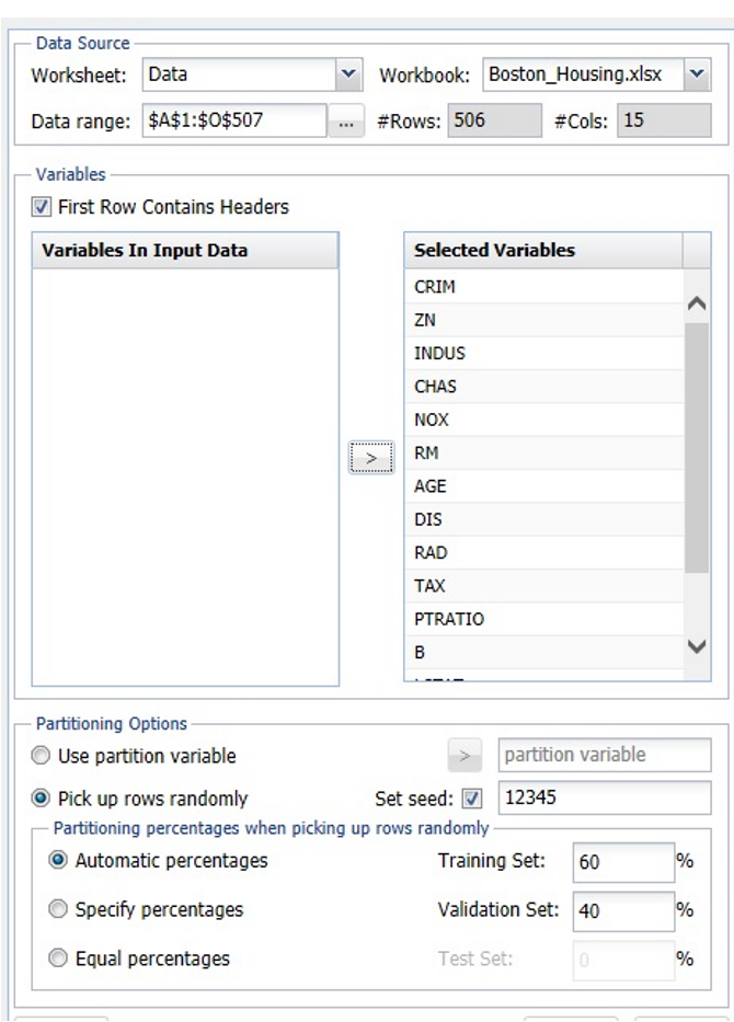
First, we partition the data into training and validation sets using the Standard Data Partition defaults with percentages of 60% of the data randomly allocated to the Training Set and 40% of the data randomly allocated to the Validation Set. For more information on partitioning a dataset, see the Analytic Solver Data Science Partitioning chapter.
Click Predict – Neural Network – Automatic on the Data Science ribbon. The Neural Network Regression Data tab appears.
Select MEDV as the Output variable, CHAS as the Categorical Variable, and the remaining variables as Selected Variables (except the CAT.MEDV and Record ID variables). The last variable, CAT.MEDV, is a discrete classification of the MEDV variable and will not be used in this example.
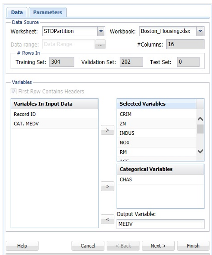
Click Next to advance to the Parameters tab.
When a neural network with automatic architecture is created, several networks are run with increasing complexity in the architecture. The networks are limited to 2 hidden layers and the number of hidden neurons in each layer is bounded by UB1 = (#features + 1) * 2/3 on the 1st layer and UB2 = (UB1 + 1) * 2/3 on the 2nd layer. For this example, select Automatic Architecture. See below for an example on specifying the number of layers when manually defining the network architecture.
First, all networks are trained with 1 hidden layer with the number of nodes not exceeding the UB1 bounds, then a second layer is added and a 2 – layer architecture is tried until the UB2 limit is satisfied.
The limit on the total number of trained networks is the minimum of 100 and (UB1 * (1+UB2)). In this dataset, there are 13 features in the model giving the following bounds:
UB1 = Floor ((13 + 1) * 2/3) = 9.33 ~ 9
UB2 = Floor ((9 + 1) * 2/3) = 6.67 ~ 6
(Floor: Rounds a number down to the nearest multiple of significance.)
# Networks Trained = MIN {100, (9 * (1 + 6)} = 63
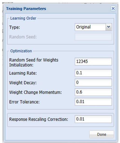
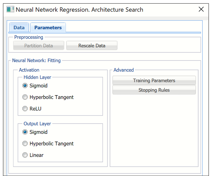
Users can now change both the Training Parameters and Stopping Rules for the Neural Network. Click Training Parameters to open the Training Parameters dialog. For information on these parameters, please see the Options section that occurs later in this chapter. For now, click Done to accept the default settings and close the dialog.
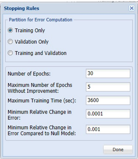
Click Stopping Rules to open the Stopping Rules dialog. Here users can specify a comprehensive set of rules for stopping the algorithm early plus cross-validation on the training error. For more information on these options, please see the Options section that appears later on in this chapter. For now, click Done to accept the default settings and close the dialog.
Keep the defaults for both Hidden Layer and Output Layer. See the Neural Network Regression Options section below for more information on these options.
Click Finish.
Click the NNP_Output tab.
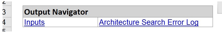
The top section includes the Output Navigator which can be used to quickly navigate to various sections of the output. The Data, Variables, and Parameters/Options sections of the output all reflect inputs chosen by the user.
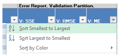
Scroll down to the Error Report, a portion is shown below. This report displays each network created by the Automatic Architecture algorithm and can be sorted by each column by clicking the down arrow next to each column heading.
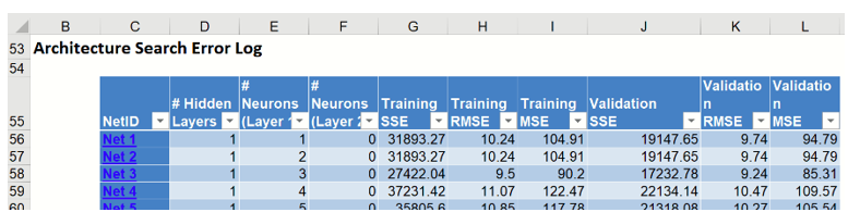
Click the down arrow next to the last column heading, Validation:MSE (Mean Standard Error for the Validation dataset), and select Sort Smallest to Largest from the menu. Note: Sorting is not supported in AnalyticSolver.com.
Immediately, the records in the table are sorted by smallest value to largest value according to the Validation: MSE values.
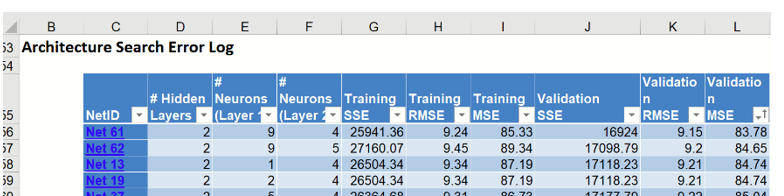
Since this column is the average residual error, the error closest to 0 would be the record with the “best” average error, or lowest residual error. Take a look at Net ID 61 which has the lowest average error in the validation dataset. This network contains 2 hidden layers containing 9 neurons in the first hidden layer and 4 neurons in the 2nd hidden layer. The Sum of Squared Error for this network is 25, 941.36 in the Training set and 16924.00 in the Validation set. Note that the number of networks trained is 63 or MIN {100, (9 * (1 + 6)} = 63 (as discussed above). Click the any of the 63 hyperlinks to open the Neural Network Regression Data tab. Click Finish to run the Neural Network Regression method using the input and option settings for the ID selected.
Read on below for the last choice in Neural Network Regression methods, creating a Neural Network, manually.