More on Introducing Uncertainty
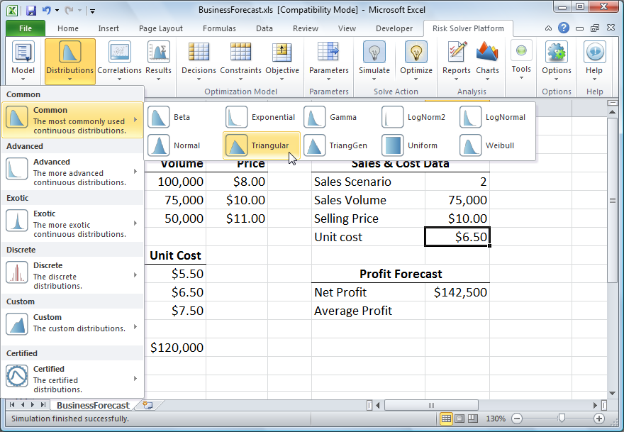
So far, we've modified our spreadsheet model to introduce uncertainty for Sales Volume at cell F5 and Selling Price at F6. Now we'll deal with Unit Cost. We have not just three, but many possible values for this variable: It can be anywhere from $5.50 to $7.50, with a most likely cost of $6.50. A crude but effective way to model this is to use a triangular distribution. Risk Solver provides a function called PsiTriangular() for this distribution.
With cell F7 (representing Unit Cost) selected, from the Risk Solver Ribbon we click the Distributions button and then select Triangular from the Common distributions gallery. (Unlike a discrete distribution, a sample drawn from a continuous distribution can be any numeric value, such as 5.8 or 6.01, in a range.)
Risk Solver displays the Uncertain Variable dialog with a chart of the triangular distribution -- initially with parameters: min 0, likely 1 and max 3. We want to edit these parameters -- but instead of entering fixed numbers, we'll use the range selector icon at the right of each field to select cells containing the parameters: min B9 ($5.50), likely B10 ($6.50) and max B11 ($7.50). This means that on each trial, we'll draw a number between $5.50 and $7.50, where $6.50 is the most likely value to be drawn -- as shown in the chart of the triangular distribution below. Hence $6.45 and $6.55 are more likely than $5.55 or $7.45 -- but any of these and other numbers has a chance of being drawn on each trial. When we click the Save icon in the dialog toolbar, a formula =PsiTriangular(B9,B10,B11) is written to F7. (Note that you could also type the formula =PsiTriangular(B9,B10,B11) in cell F7.) We now have a second uncertain variable in our model.
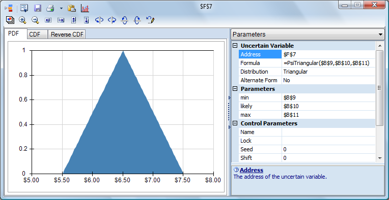
Next, we'll move on to define an Uncertain Function. But we can do much more than shown here with the Uncertain Variable dialog: The view above shows all of its panes open. You can browse different distributions, shift and truncate a distribution, see each distribution's Probability Density Function (PDF), Cumulative Density Function (CDF) or Reverse CDF, see statistics and percentiles for the distribution, automatically fit a distribution to user-supplied data, and customize the chart.
< Back to: Monte Carlo Simulation Tutorial Start Next: Uncertain Functions and Statistics >