This example illustrates how to use Analytic Solver's Holt Winters Smoothing technique to uncover trends in the time series dataset Airpass.xlsx. This example will create three different forecasts, one for each Holt Winters model type, beginning with Multiplicative.
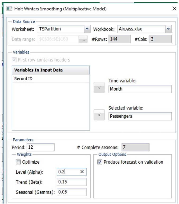
Click back to the TSPartition worksheet and click Smoothing – Holt Winters – Multiplicative to open the Holt Winters Smoothing (Multiplicative Model) dialog.
Select Month for the Time variable, if not already selected, and Passengers for Selected variable.
Since our dataset contains airline passengers, we can assume some seasonality exists in the data since most passengers fly during the summer and holiday months (i.e. December).
It takes a full 12 months to complete the seasonality cycle so enter 12 for Period, # Complete seasons is automatically entered with the number 7. This example will use the defaults for the three parameters: Alpha, Beta, and Gamma.
Values between 0 and 1 can be entered for each parameter. As with Exponential Smoothing, values close to 1 will result in the most recent observations being weighted more than earlier observations.
In the Multiplicative model, it is assumed that the values for the different seasons differ by percentage amounts.
Produce Forecast on validation is selected by default.
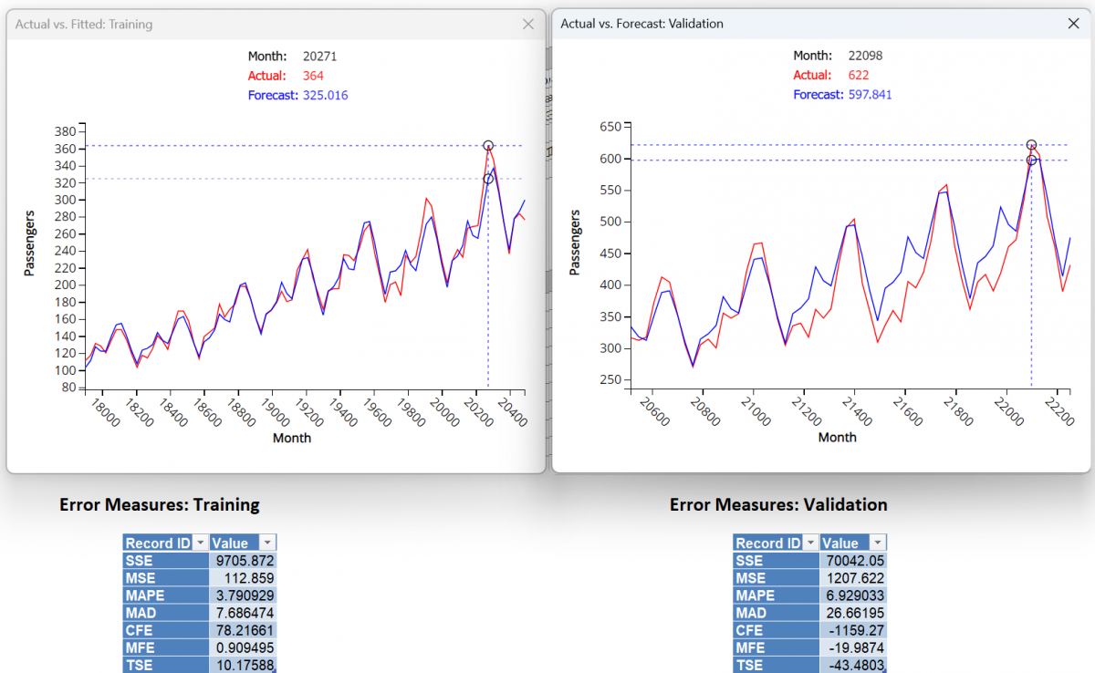
Click OK to run the smoothing technique. The results of the smoothing technique, MulHoltWinters and MulHoltWinters_Stored, are inserted to the right of the TSPartition worksheet. For more information on MulHoltWinters_Stored, see the chapter “Scoring New Data” within the Analytic Solver User Guide.
Note: To view these two charts in the Cloud app, click the Charts icon on the Ribbon, select MulHoltWinters for Worksheet and Time Series Training Data or Time Series Validation Data for Chart.
If you inspect the MSE (Mean Squared Error) term in the Error Measures (Validation) table, you’ll see that this value is fairly high. In addition, the peaks for the Forecast data appear to lag behind the peaks in the Validation data. This suggests that our Trend (Beta) parameter is too large.
Let’s go back and try the Multiplicative method one more time using the Optimize parameter. This parameter will choose the best values for the Alpha, Trend, and Seasonal parameters based on the Forecasting Mean Squared Error. It is recommended that this feature be used carefully as this option can lead to overfitting. An overfit model rarely exhibits high predictive accuracy in the validation set.
Click Smoothing – Holt-Winters – Multiplicative on the Data Science ribbon.
We will again select Passengers for Selected Variable (if not already selected) and 12 for Period. Produce Forecast on Validation is selected by default. This time we’ll also select the Optimize parameter.
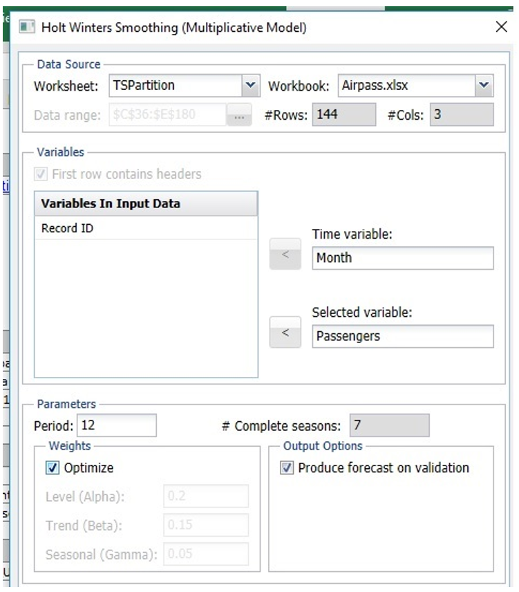
Afterwards, click OK to proceed with the smoothing technique.
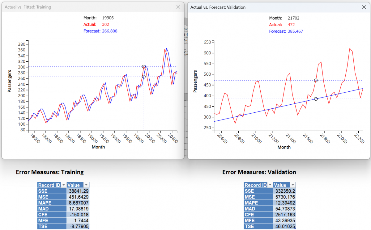
MulHoltWinters1 is inserted to the right.

The Parameters/Options table gives us the parameter settings as chosen by the Optimize feature for Alpha (0.858), Beta (0.003) and Gamma (0.917). (Recall that the default settings as 0.20 (Alpha), 0.15 (Beta) and 0.05 (Seasonal).) Scroll down to find the Training and Validation Error Measures.
Note: To view these two charts in the Cloud app, click the Charts icon on the Ribbon, select MulHoltWinters1 for Worksheet and Time Series Training Data or Time Series Validation Data for Chart.
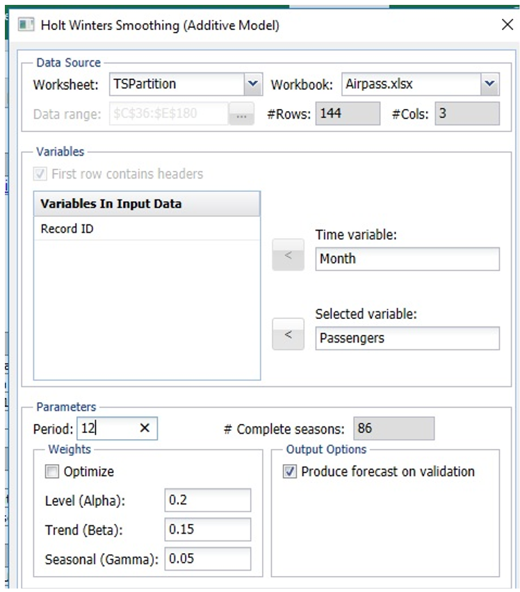
Now let’s create a new model using the Additive model. This technique assumes the values for the different seasons differ by a constant amount. Click back to the TSPartition sheet, then click Smoothing – Holt Winters – Additive to open the Holt Winters Smoothing (Additive Model) dialog.
Select Month for Time Variable, if not already selected, and Passengers for Selected variable. Again, enter 12 for Period. Produce Forecast on validation is selected by default.
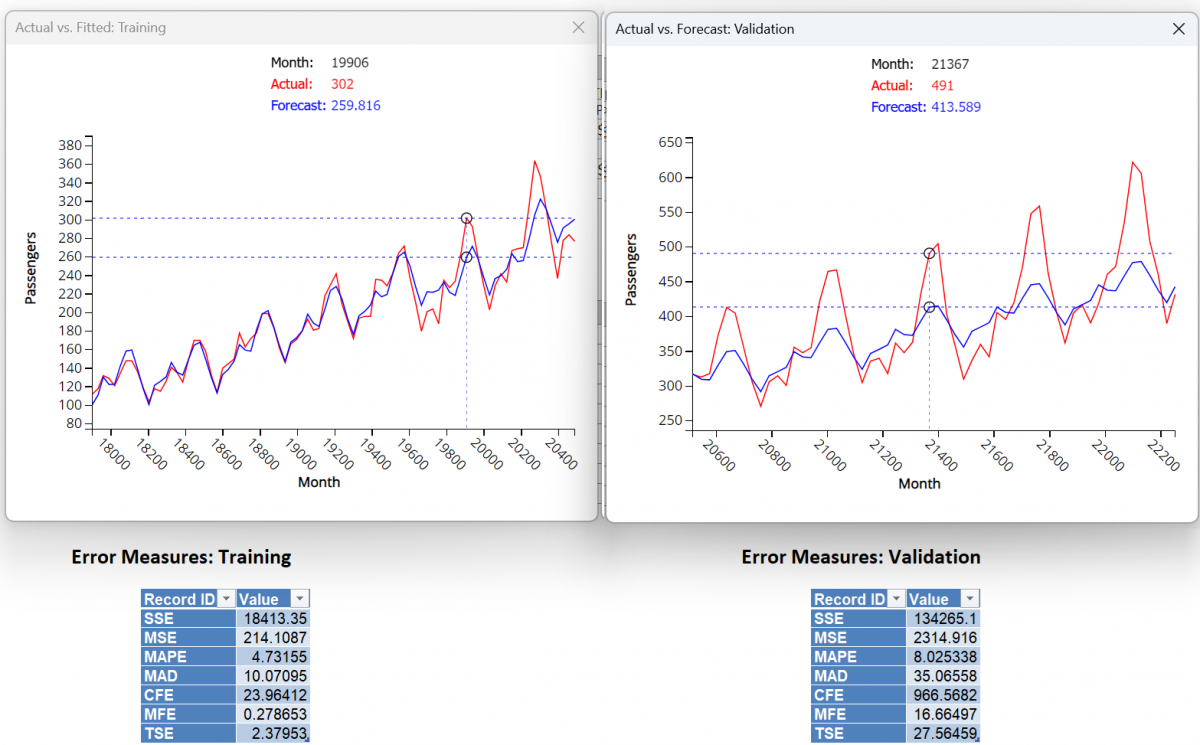
Click OK to run the smoothing technique. AddHoltWinters and AddHoltWinters_Stored will be inserted right of the TSPartition worksheet. For more information on AddHoltWinters_Stored, see the chapter, “Scoring New Data” within the Analytic Solver User Guide.
Click a point anywhere on the function to compare Actual vs. Forecasted at the top of the graph.
Note: To view these two charts in the Cloud app, click the Charts icon on the Ribbon, select AddHoltWinters for Worksheet and Time Series Training Data or Time Series Validation Data for Chart.
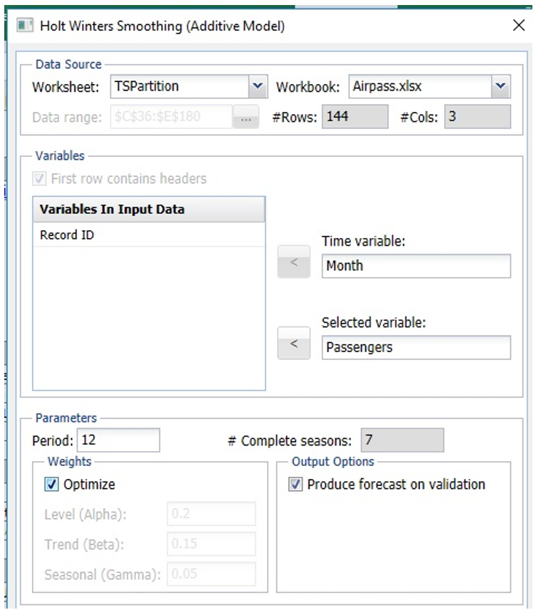
Let’s try the Additive model again using the Optimize feature. Click back to TSPartition and then click Smoothing – Holt-Winters – Additive on the Data Science ribbon.
Select Month for Time Variable and Passengers for Selected Variable, then 12 for Period. Produce Forecast on Validation is selected by default. Select Optimize to run the Optimize algorithm which will pick the best values for the three parameters, Alpha, Beta, and Gamma.
Click OK, then click the, AddHoltWinters1, tab.
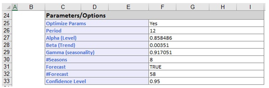
Notice the parameter values chosen by the Optimize algorithm were 0.858 for Alpha, .00351 for Beta, and 0.917 for Gamma. Scroll down to view the results of the model fitting.
Note: To view these two charts in the Cloud app, click the Charts icon on the Ribbon, select AddHoltWinters1 for Worksheet and Time Series Training Data or Time Series Validation Data for Chart.
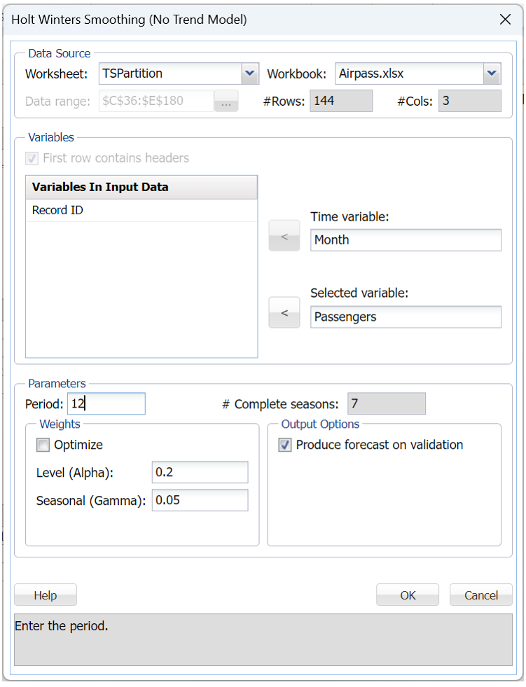
The last Holt Winters model should be used with time series that contain seasonality, but no trends. Click back to TSPartition, then click Smoothing – Holt Winters – No Trend to open the Holt Winters Smoothing (No trend Model) dialog.
Select Month for Time variable unless already selected. Select Passengers as the Selected variable. Enter 12 for Period. Produce Forecast on validation is selected by default. Notice that the trend parameter is missing. Values for Alpha and Gamma can range from 0 to 1. A value of 1 for each parameter will assign higher weights to the most recent observations and lower weights to the earlier observations. This example will accept the default values.
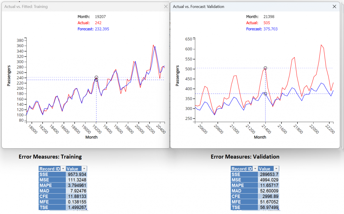
Click OK to run the smoothing technique. NoTrendHoltWinters and NoTrendHoltWinters_Stored are right of the TSPartition worksheet.
Note: To view these two charts in the Cloud app, click the Charts icon on the Ribbon, select NoTrendHoltWinters for Worksheet and Time Series Training Data or Time Series Validation Data for Chart.
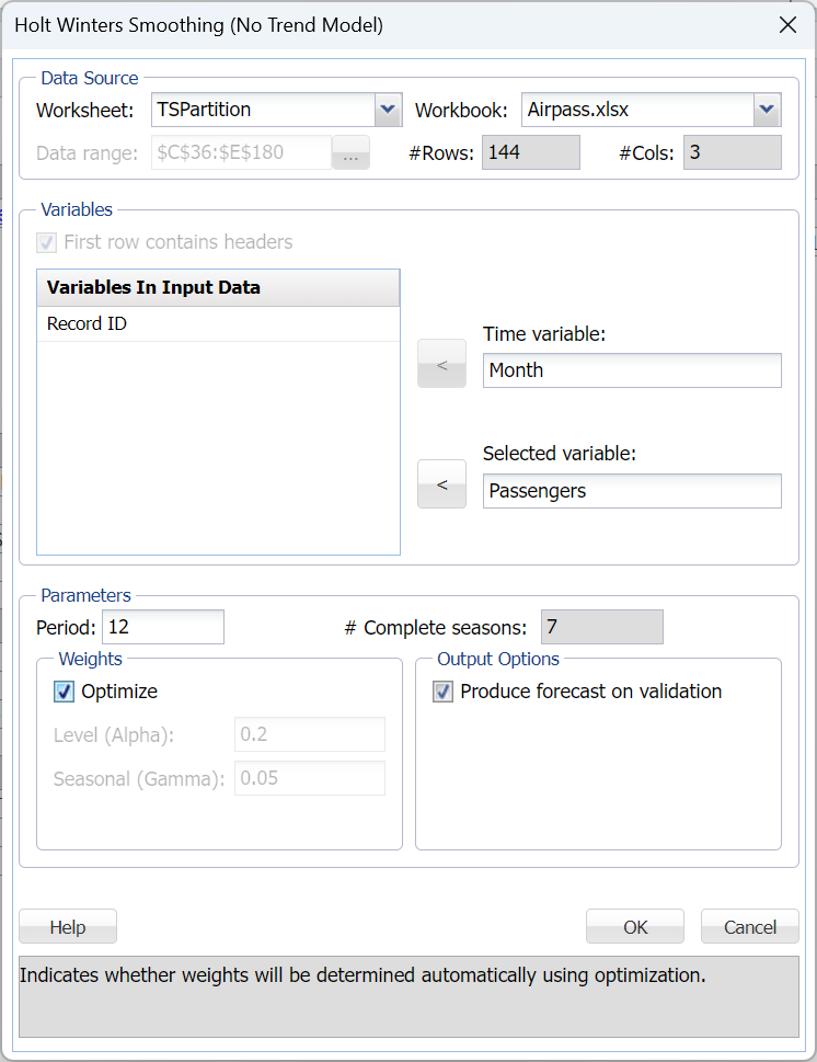
Let’s try the No Trend model again using the Optimize feature. Click back to TSPartition, then click Smoothing – Holt-Winters – No Trend on the Data Science ribbon.
Select Month for Time variable, unless already selected, and Passengers for Selected variable, 12 for Period. Produce Forecast on Validation is selected by default. Select Optimize to run the Optimize algorithm which will pick the best values for the two parameters, Alpha and Gamma.
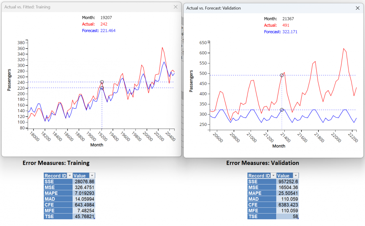
Click OK. NoTrendHoltWinters1 is inserted to the right.
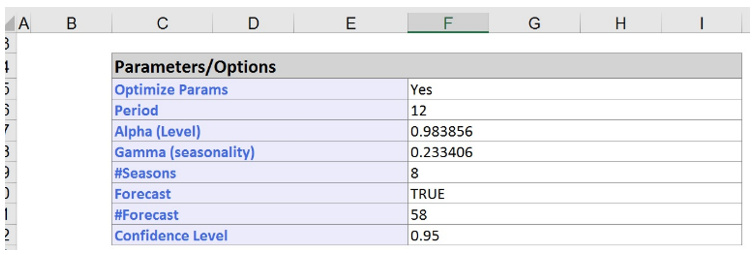
Notice the parameter values chosen by the Optimize algorithm were 0.984 for Alpha and 0.233 for Gamma. Scroll down to view the results of the model fitting.

Note: To view these two charts in the Cloud app, click the Charts icon on the Ribbon, select NoTrendHoltWinters for Worksheet and Time Series Training Data or Time Series Validation Data for Chart.