This example uses the text files within the Text Mining Example Documents.zip archive file to illustrate how to use Analytic Solver Data Science’s Text Mining tool. These documents were selected from the well-known text dataset (downloadable from here) which consists of 20,000 messages, collected from 20 different internet newsgroups. We selected about 1,200 of these messages that were posted to two interest groups, Autos and Electronics (about 500 documents from each).
Note: Analytic Solver Cloud does not currently support importing from a file folder.
Importing from a File Folder
The Text Mining Example Documents.zip archive file is located at C:\Program Files\Frontline Systems\Analytic Solver Platform\Datasets. Unzip the contents of this file to a location of your choice. Four folders will be created beneath Text Mining Example Documents: Autos, Electronics, Additional Autos and Additional Electronics. One thousand, two hundred short text files will be extracted to the location chosen. This example is based on the text dataset at http://www.cs.cmu.edu/afs/cs/project/theo-20/www/data/news20.html, which consists of 20,000 messages, collected from 20 different netnews newsgroups. We selected about 1,200 of these messages that were posted to two interest groups, for Autos and Electronics (about 50% in each).
Select Get Data – File Folder to open the Import From File System dialog.
At the top of the dialog, click Browse… to navigate to the Autos subfolder (C:\Program Files\Frontline Systems\Analytic Solver Platform\Datasets\Text Mining Example Documents\Autos). Set the File Type to All Files (*.*), then select all files in the folder and click the Open button. The files will appear in the left listbox under Files. Click the >> button to move the files from the Files listbox to the Selected Files listbox. Now repeat these steps for the Electronics subfolder. When these steps are completed, 985 files will appear under Selected Files.
Select Sample from selected files to enable the Sampling Options. Text Miner will perform sampling from the files in the Selected Files field. Enter 300 for Desired sample size while leaving the default settings for Simple random sampling and Set Seed.
Note: If you are using the educational version of Analytic Solver Data Science, enter "100" for Desired Sample Size. This is the upper limit for the number of files supported when sampling from a file system when using Analytic Solver Data Science. For a complete list of the capabilities of Analytic Solver Data Science and Analytic Solver Data Science for Education, click here.
Text Miner will select 300 files using Simple random sampling with a seed value of 12345. Under Output, leave the default setting of Write file paths. Rather than writing out the file contents into the report, Text Miner will include the file paths.
Note: Currently, Analytic Solver Data Science only supports the import of delimited text files. A delimited text file is one in which data values are separated by a character such as quotation marks, commas or tabs. These characters define a beginning and end of a string of text.

Click OK. The output FileSampling will be inserted into the Data Science task pane, with contents similar to that shown on the next page.
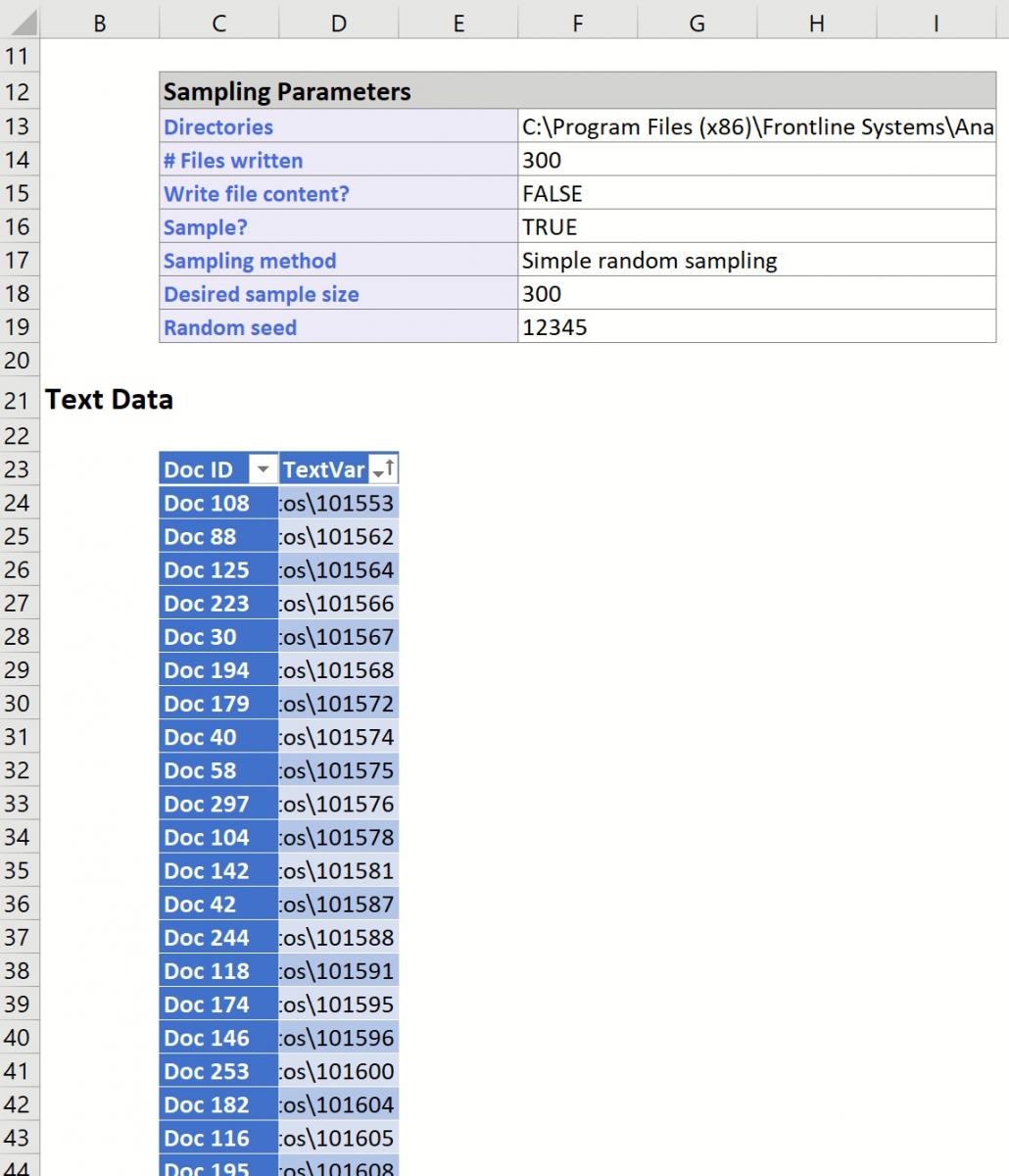
The Data portion of the report displays the selections we made on the Import From File System dialog. Here we see the path of the directories, the number of files written, our choice to write the paths or contents (File Paths), the sampling method, the desired sample size, the actual size of the sample, and the seed value (12345).
Underneath the Data portion are paths to the 300 text files in random order that were sampled by Analytic Solver Data Science. If Write file contents had been selected, rather than Write file paths, the report would contain the RowID, File Path, and the first 32,767 characters present in the document.
Following is an example of a document that appeared in the Electronics news group. Note the appearance of email addresses, From, and Subject lines. All three appear in each document.

The selected file paths are now in random order, but we need to categorize the Autos and Electronics files to be able to identify them later. To do this, use Excel to sort the rows by the file path: Select columns B through D and rows 18 through 317. On the Excel ribbon, from the Data tab, from the Sort & Filter icon, select Sort to open the Sort dialog. Select column d, where the file paths are located, and click OK.
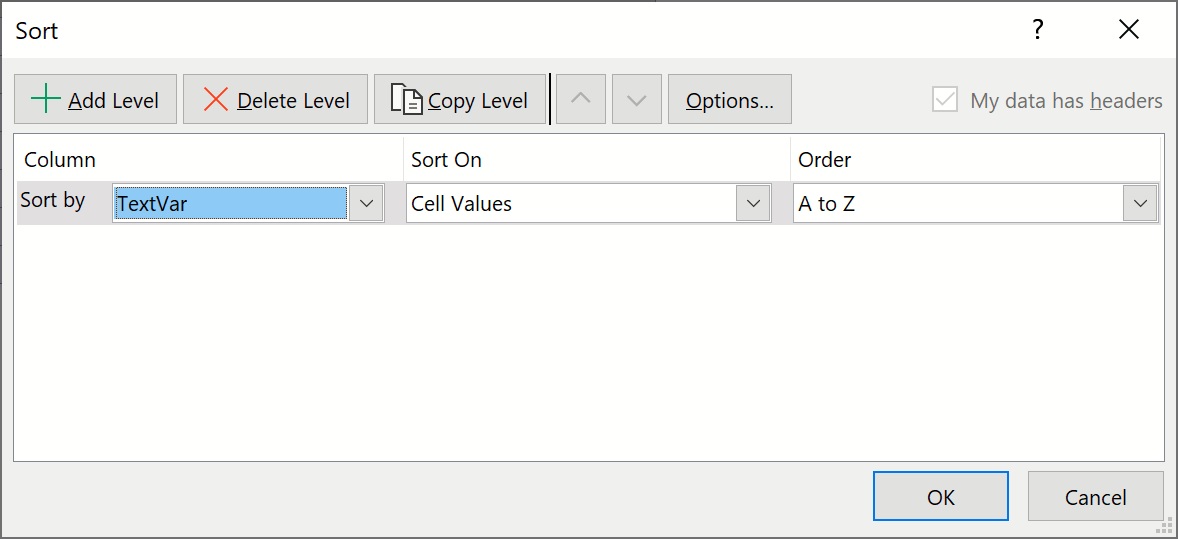
The file paths are now sorted between Autos and Electronic files.

Using Text Miner
Click the Text icon to bring up the Text Miner dialog.
Data Source tab
Confirm that FileSampling is selected for Worksheet. Select TextVar in the Variables listbox, and click the upper > button to move it to the Selected Text Variables listbox. By doing so, we are selecting the text in the documents as input to the Text Miner model. Ensure that “Text variables contain file paths” is checked.
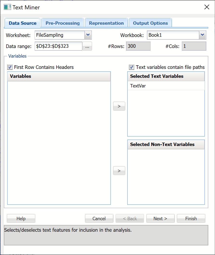
Click the Next button, or click the Pre-Processing tab at the top. (The Models tab can be used to process new documents using an existing text mining model. Since we do not have an existing model we’ll leave this tab blank.)
Pre-Processing Tab
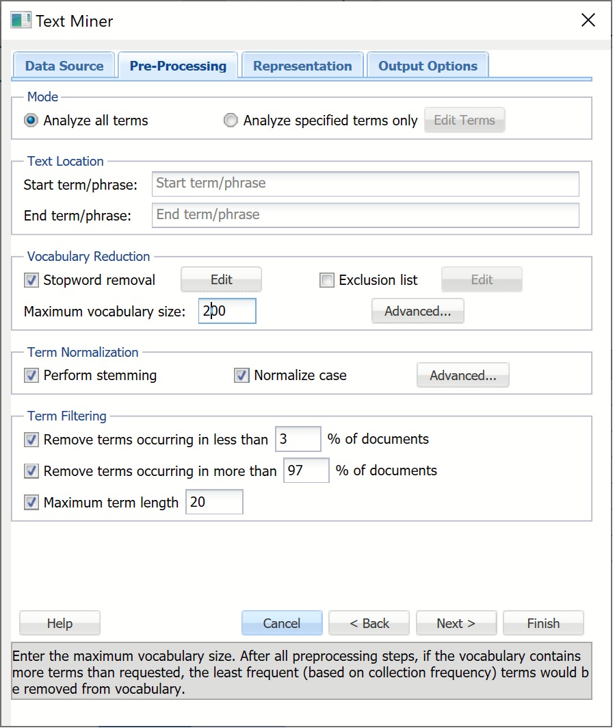
Leave the default setting for Analyze all terms selected under Mode. When this option is selected, Text Miner will examine all terms in the document. A “term” is defined as an individual entity in the text, which may or may not be an English word. A term can be a word, number, email, url, etc. terms are separated by all possible delimiting characters (i.e. \, ?, ', `, ~, |, \r, \n, \t, :, !, @, #, $, %, ^, &, *, (, ), [, ], {, }, <>,_, ;, =, -, +, \) with some exceptions related to stopwords, synonyms, exclusion terms and boilerplate normalization (URLs, emails, monetary amounts, etc.). Text Miner will not tokenize on these delimiters.
Note: Exceptions are related not to how terms are separated but as to whether they are split based on the delimiter. For example: URL's contain many characters such as "/", ";", etc. Text Miner will not tokenize on these characters in the URL but will consider the URL as a whole and will remove the URL if selected for removal. (See below for more information.)
If Analyze specified terms only is selected, the Edit Terms button will be enabled. If you click this button, the Edit Exclusive Terms dialog opens. Here you can add and remove terms to be considered for text mining. All other terms will be disregarded. For example, if we wanted to mine each document for a specific part name such as “alternator” we would click Add Term on the Edit Exclusive Terms dialog, then replace “New term” with “alternator” and click Done to return to the Pre-Processing dialog. During the text mining process, Text Miner would analyze each document for the term “alternator”, excluding all other terms.
Leave both Start term/phrase and End term/phrase empty under Text Location. If this option is used, text appearing before the first occurrence of the Start Phrase will be disregarded and similarly, text appearing after End Phrase (if used) will be disregarded. For example, if text mining the transcripts from a Live Chat service, you would not be particularly interested in any text appearing before the heading “Chat Transcript” or after the heading “End of Chat Transcript”. Thus you would enter “Chat Transcript” into the Start Phrase field and “End of Chat Transcript” into the End Phrase field.
Leave the default setting for Stopword removal. Click Edit to view a list of commonly used words that will be removed from the documents during pre-processing. To remove a word from the Stopword list, simply highlight the desired word, then click Remove Stopword. To add a new word to the list, click Add Stopword, a new term “stopword” will be added. Double click to edit.
Text Miner also allows additional stopwords to be added or existing to be removed via a text document (*.txt) by using the Browse button to navigate to the file. Terms in the text document can be separated by a space, a comma, or both. If we were supplying our three terms in a text document, rather than in the Edit Stopwords dialog, the terms could be listed as: subject emailterm from or subject,emailterm,from or subject, emailterm, from. If we had a large list of additional stopwords, this would be the preferred way to enter the terms.

Click Advanced in the Term Normalization group to open the Term Normalization – Advanced dialog. Select all options as shown below. Then click Done. This dialog allows us to indicate to Text Miner, that
- If stemming reduced term length to 2 or less characters, disregard the term (Minimum stemmed term length).
- HTML tags, and the text enclosed, will be removed entirely. HTML tags and text contained inside these tags often contain technical, computer-generated information that is not typically relevant to the goal of the text mining application.
- URLs will be replaced with the term, “urltoken”. Specific form of URLs do not normally add any meaning, but it is sometimes interesting to know how many URLs are included in a document.
- Email addresses will be replaced with the term, “emailtoken”. Since the documents in our collection all contain a great many email addresses (and the distinction between the different emails often has little use in Text Mining), these email addresses will be replaced with the term “emailtoken”.
- Numbers will be replaced with the term, “numbertoken”.
- Monetary amounts will be substituted with the term, “moneytoken”.

Recall that when we inspected an email from the document collection we saw several terms such as “subject”, “from” and email addresses. Since all of our documents contain these terms, including them in the analysis will not provide any benefit and could bias the analysis. As a result, we will exclude these terms from all documents by selecting Exclusion list then clicking Edit. The Edit Exclusion List dialog opens. Click Add Exclusion Term. The label “exclusionterm” is added. Click to edit and change to “subject”. Then repeat these same steps to add the term “from”.
We can take the email issue one step further and completely remove the term “emailtoken” from the collection. Click Add Exclusion Term and edit “exclusionterm” to “emailtoken”.
To remove a term from the exclusion list, highlight the term and click Remove Exclusion Term.
We could have also entered these terms into a text document (*.txt) and added the terms all at once by using the Browse button to navigate to the file and import the list. Terms in the text document can be separated by a space, a comma, or both. If, for example we were supplying excluded terms in a document rather than in the Edit Exclusion List dialog, we would enter the terms as: subject emailtoken from, or subject,emailtoken,from, or subject, emailtoken, from. If we had a large list of terms to be excluded, this would be the preferred way to enter the terms.

Click Done to close the dialog and return to the Pre-Processing dialog.
Text Miner allows the combining of synonyms and full phrases by clicking Advanced under Vocabulary Reduction. Select Synonym reduction at the top of the dialog to replace synonyms such as car, automobile, convertible, vehicle, sedan, coupe, subcompact, and jeep with auto. Click Add Synonym and replace rootterm with auto, then replace synonym list with car, automobile, convertible, vehicle, sedan, coupe (without the parenthesis). During pre-processing, XLMiner replaces the terms car, automobile, convertible, vehicle, sedan, coupe, subcompact, and jeep with the term auto. To remove a synonym from the list, highlight the term and click Remove Synonym.
If adding synonyms from a text file, each line must be of the form rootterm:synonymlist, or using our example: auto:car automobile convertible vehicle sedan coup or auto:car,automobile,convertible,vehicle,sedan,coup. Note that separation between the terms in the synonym list must be either a space, a comma, or both. If there were a large list of synonyms, this would be the preferred way to enter the terms.
Text Miner allows the combining of words into phrases that indicate a singular meaning such as station wagon, which refers to a specific type of car rather than two distinct tokens -- station and wagon. To add a phrase in the Vocabulary Reduction - Advanced dialog, select Phrase reduction and click Add Phrase. When the term phrasetoken appears, click to edit and enter wagon. Click phrase to edit and enter station wagon. If supplying phrases through a text file (*.txt), each line of the file must be of the form phrasetoken:phrase or using our example, wagon:station wagon. With a large list of phrases, this would be the preferred way to enter the terms.

Enter 200 for Maximum Vocabulary Size. Text Miner will reduce the number of terms in the final vocabulary to the top 200 most frequently occurring in the collection.
Leave Perform stemming at the selected default. Stemming is the practice of stripping words down to their “stems” or “roots”, for example, stemming terms such as “argue”, “argued”, “argues”, “arguing”, and “argus” would result in the stem “argu. However “argument” and “arguments” would stem to “argument”. The stemming algorithm utilized in Text Miner is “smart” in the sense that while “running” would be stemmed to “run”, “runner” would not. . Text Miner uses the Porter Stemmer 2 algorithm for the English Language. For more information on this algorithm, please see the Webpage: http://tartarus.org/martin/PorterStemmer/
Leave the default selection for Normalize case. When this option is checked, Text Miner converts all text to a consistent (lower) case, so that Term, term, TERM, etc. are all normalized to a single token “term” before any processing, rather than creating three independent tokens with different case. This simple method can dramatically affect the frequency distributions of the corpus, leading to biased results.
Enter 3 for Remove terms occurring in less than _% of documents and 97 for Remove terms occurring in more than _% of documents. For many text mining applications, the goal is to identify terms that are useful for discriminating between documents. If a particular term occurs in all or almost all documents, it may not be possible to highlight the differences. If a term occurs in very few documents, it will often indicate great specificity of this term, which is not very useful for some Text Mining purposes.
Enter 20 for Maximum term length. Terms that contain more than 20 characters will be excluded from the text mining analysis and will not be present in the final reports. This option can be extremely useful for removing some parts of text which are not actual English words, for example, URLs or computer-generated tokens, or to exclude very rare terms such as Latin species or disease names, i.e. Pneumonoultramicroscopicsilicovolcanoconiosis.
Click Next to advance to the Representation tab or simply click Representation at the top.
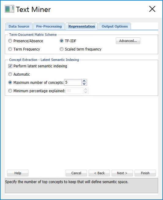
Representation Tab
Keep the default selection of TF-IDF (Term Frequency – Inverse Document Frequency) for Term-Document Matrix Scheme. A term-document matrix is a matrix that displays the frequency-based information of terms occurring in a document or collection of documents. Each column is assigned a term and each row a document. If a term appears in a document, a weight is placed in the corresponding column indicating the term’s importance or contribution. Text Miner offers four different commonly used methods of weighting scheme used to represent each value in the matrix: Presence/Absence, Term Frequency, TF-IDF (the default) and Scaled term frequency. If Presence/Absence is selected, Text Miner will enter a 1 in the corresponding row/column if the term appears in the document and 0 otherwise. This matrix scheme does not take into account the number of times the term occurs in each document. If Term Frequency is selected, Text Miner will count the number of times the term appears in the document and enter this value into the corresponding row/column in the matrix. The default setting – Term Frequency – Inverse Document Frequency (TF-IDF) is the product of scaled term frequency and inverse document frequency. Inverse document frequency is calculated by taking the logarithm of the total number of documents divided by the number of documents that contain the term. A high value for TF-IDF indicates that a term that does not occur frequently in the collection of documents taken as a whole, appears quite frequently in the specified document. A TF-IDF value close to 0 indicates that the term appears frequently in the collection or rarely in a specific document. If Scaled term frequency is selected, Text Miner will normalize (bring to the same scale) the number of occurrences of a term in the documents (see the table below).
It’s also possible to create your own scheme by clicking the Advanced command button to open the Term Document Matrix – Advanced dialog. Here users can select their own choices for local weighting, global weighting, and normalization. Please see the table below for definitions regarding options for Term Frequency, Document Frequency and Normalization.

Leave Perform latent semantic indexing selected (the default). When this option is selected, Text Miner will use Latent Semantic Indexing (LSI) to detect patterns in the associations between terms and concepts to discover the meaning of the document.
The statistics produced and displayed in the Term-Document Matrix contain basic information on the frequency of terms appearing in the document collection. With this information we can “rank” the significance or importance of these terms relative to the collection and particular document. Latent Semantic Indexing, in comparison, uses singular value decomposition (SVD) to map the terms and documents into a common space to find patterns and relationships. For example: if we inspected our document collection, we might find that each time the term “alternator” appeared in an automobile document, the document also included the terms “battery” and “headlights”. Or each time the term “brake” appeared in an automobile document, the terms “pads” and “squeaky” also appeared. However there is no detectable pattern regarding the use of the terms “alternator” and “brake”. Documents including “alternator” might not include “brake” and documents including “brake” might not include “alternator”. Our four terms, battery, headlights, pads, and squeaky describe two different automobile repair issues: failing brakes and a bad alternator. Latent Semantic Indexing will attempt to 1. Distinguish between these two different topics, 2. Identify the documents that deal with faulty brakes, alternator problems or both and 3. Map the terms into a common semantic space using singular value decomposition. SVD is a tool used by Text Miner to extract concepts that explain the main dimensions of meaning of the documents in the collection. The results of LSA are usually hard to examine because the construction of the concept representations will not be fully explained. Interpreting these results is actually more of an art, than a science. However, Text Miner provides several visualizations that simplify this process greatly.
Select Maximum number of concepts and increment the counter to 20. Doing so will tell Text Miner to retain the top 20 of the most significant concepts. If Automatic is selected, Text Miner will calculate the importance of each concept, take the difference between each and report any concepts above the largest difference. For example if three concepts were identified (Concept1, Concept2, and Concept3) and given importance factors of 10, 8, and 2, respectively, Tex Miner would keep Concept1 and Concept2 since the difference between Concept2 and Concept 3 (8-2=6) is larger than the difference between Concept1 and Concept2 (10-8=2). If Minimum percentage explained is selected, Text Miner will identify the concepts with singular values that, when taken together, sum to the minimum percentage explained, 90% is the default.
Click Next or the Output Options tab.
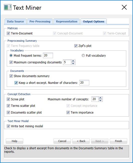
Options Tab
Keep Term-Document and Concept-Document selected under Matrices (the default) and select Term-Concept to print each matrix in the output. The Term-Document matrix displays the terms across the top of the matrix and the documents down the left side of the matrix. The Concept – Document and Term – Concept matrices are output from the Perform latent semantic indexing option that we selected on the Representation tab. In the first matrix, Concept – Document, 20 concepts will be listed across the top of the matrix and the documents will be listed down the left side of the matrix. The values in this matrix represent concept coordinates in the identified semantic space. In the Term-Concept matrix, the terms will be listed across the top of the matrix and the concepts will be listed down the left side of the matrix. The values in this matrix represent terms in the extracted semantic space.
Keep Term frequency table selected (the default) under Preprocessing Summary and select Zipf’s plot. Increase the Most frequent terms to 20 and select Maximum corresponding documents. The Term frequency table will include the top 20 most frequently occurring terms. The first column, Collection Frequency, displays the number of times the term appears in the collection. The 2nd column, Document Frequency, displays the number of documents that include the term. The third column, Top Documents, displays the top 5 documents where the corresponding term appears the most frequently. The Zipf Plot graphs the document frequency against the term ranks in descending order of frequency.. Zipf’s law states that the frequency of terms used in a free-form text drops exponentially, i.e. that people tend to use a relatively small number of words extremely frequently and use a large number of words very rarely.
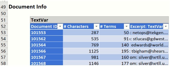
Keep Show documents summary selected and check Keep a short excerpt. under Documents. Text Miner will produce a table displaying the document ID, length of the document, number of terms and 20 characters of the text of the document.
Select all plots under Concept Extraction to produce various plots in the output. Select Write text mining model under Text Miner Model to write the model to an output sheet.
Click the Finish button to run the Text Mining analysis. Result worksheets are inserted to the right.
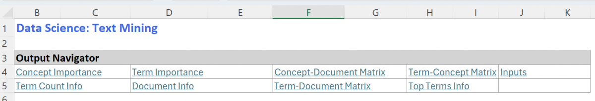
Output Results
The Output Navigator appears at the top of each output worksheet. Clicking any of these links will allow you to "jump" to the desired output.
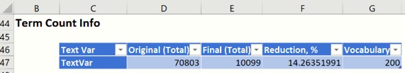
Term Count and Document Info
Select the TM_Output tab. The Term Count table shows that the original term count in the documents was reduced by 14.26% by the removal of stopwords, excluded terms, synonyms, phrase removal and other specified preprocessing procedures.
Scroll down to the Documents table. This table lists each Document with its length, number of terms, and if Keep a short excerpt is selected on the Output Options tab and a value is present for Number of characters, then an excerpt from each document will be displayed.
Term-Document Matrix
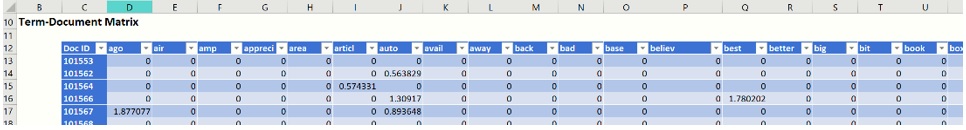
Click TM_TDM, to display the Term – Document Matrix. As discussed above, this matrix lists the 200 most frequently appearing terms across the top and the document IDs down the left. A portion of this table is shown below. If a term appears in a document, a weight is placed in the corresponding column indicating the importance of the term using our selection of TF-IDF on the Representation dialog.
Vocabulary Matrix
Click TM_Vocabulary to view the Final List of Terms table. This table contains the top 20 terms occurring in the document collection, the number of documents that include the term and the top 5 document IDs where the corresponding term appears most frequently. In this list we see terms such as “car”, “power”, “engine”, “drive”, and “dealer” which suggests that many of the documents, even the documents from the electronic newsgroup, were related to autos.
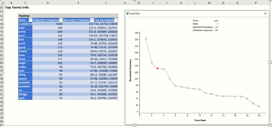
When you click on the TM_Vocabulary tab, the Zipf Plot opens. We see that our collection of documents obey the power law stated by Zipf (see above). As we move from left to right on the graph, the documents that contain the most frequently appearing terms (when ranked from most frequent to least frequent) drop quite steeply. Hover over each data point to see the detailed information about the term corresponding to this data point.
Note: To view charts in the Data Science Cloud app, click Charts on the Ribbon, select the desired worksheet, in this case TM_Vocabulary, then select the desired chart.
The term “numbertoken” is the most frequently occurring term in the document collection appearing in 223 documents (out of 300), 1,083 times total. Compare this to a less frequently occurring term such as "thing" which appears in only 64 documents and only 82 times total.
Concept Importance
Click TM_LSASummary to view the Concept Importance and Term Importance tables. The first table, the Concept Importance table, lists each concept, its singular value, the cumulative singular value and the % singular value explained. (The number of concepts extracted is the minimum of the number of documents (985) and the number of terms (limited to 200).) These values are used to determine which concepts should be used in the Concept – Document Matrix, Concept – Term Matrix and the Scree Plot according to the Users selection on the Representation tab. In this example, we entered “20” for Maximum number of concepts.
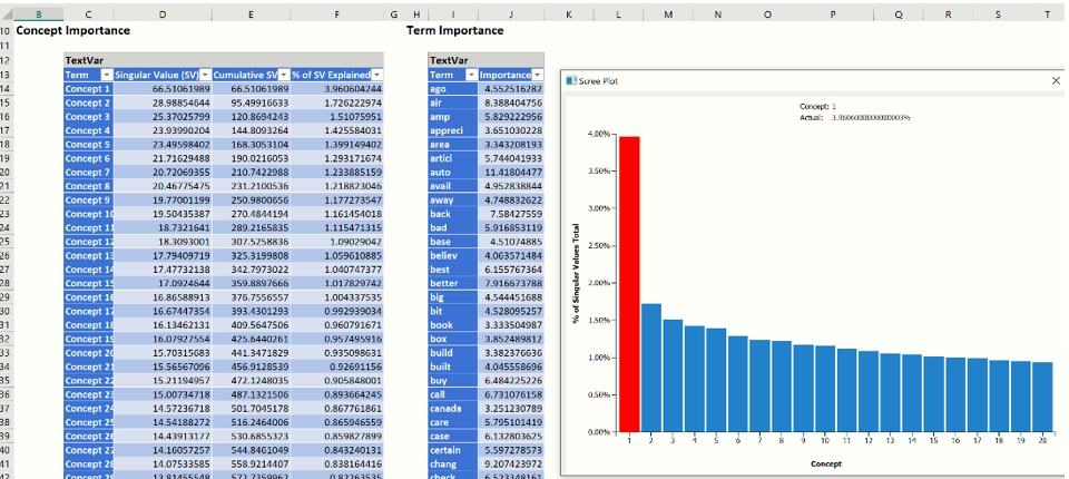
The Term Importance table lists the 200 most important terms. (To increase the number of terms from 200, enter a larger value for Maximum Vocabulary on the Pre-processing tab of Text Miner.)
When you click the TM_LSASummary tab, the Scree Plot opens. This plot gives a graphical representation of the contribution or importance of each concept. The largest “drop” or “elbow” in the plot appears between the 1st and 2nd concept. This suggests that the first top concept explains the leading topic in our collection of documents. Any remaining concepts have significantly reduced importance. However, we can always select more than 1 concept to increase the accuracy of the analysis – it is advised to examine the Concept Importance table and the “Cumulative Singular Value” in particular to identify how many top concepts capture enough information for your application.
Concept Document Matrix
Click TM_LSA_CDM to display the Concept – Document Matrix. This matrix displays the top concepts (as selected on the Representation tab) along the top of the matrix and the documents down the left side of the matrix.
When you click on the TM_LSA_CDM tab, the Concept-Document Scatter Plot opens. This graph is a visual representation of the Concept – Document matrix. Note that Analytic Solver Data Science normalizes each document representation so it lies on a unit hypersphere. Documents that appear in the middle of the plot, with concept coordinates near 0 are not explained well by either of the shown concepts. The further the magnitude of coordinate from zero, the more effect that particular concept has for the corresponding document. In fact, two documents placed at extremes of a concept (one close to -1 and other to +1) indicates strong differentiation between these documents in terms of the extracted concept. This provides means for understanding actual meaning of the concept and investigating which concepts have the largest discriminative power, when used to represent the documents from the text collection.
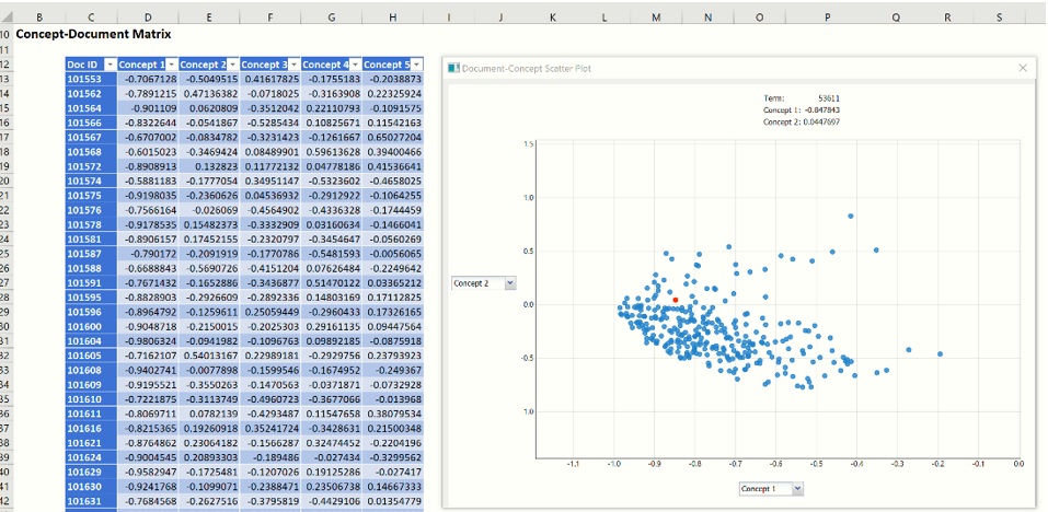
You can examine all extracted concepts by changing the axes on a scatter plot - click the down pointing arrow next to Concept 1 or the concept on the Y axis by clicking the right pointing arrow next to Concept 2. Use your touchscreen or your mouse scroll wheel to zoom in and out.
Term-Concept Matrix
Double click TM_LSA_CTM to display the Concept – Term Matrix which lists the top 5 most important concepts along the top of the matrix and the top 200 most frequently appearing terms down the side of the matrix.
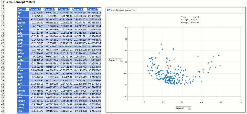
When you click on the TM_LSA-CTM tab, the Term-Concept Scatter Plot opens. This graph is a visual representation of the Concept – Term Matrix. It displays all terms from the final vocabulary in terms of two concepts. Similarly to the Concept-Document scatter plot, the Concept-Term scatter plot visualizes the distribution of vocabulary terms in the semantic space of meaning extracted with LSA. The coordinates are also normalized, so the range of axes is always [-1,1], where extreme values (close to +/-1) highlight the importance or “load” of each term to a particular concept. The terms appearing in a zero-neighborhood of concept range do not contribute much to a concept definition. In our example, if we identify a concept having a set of terms that can be divided into two groups: one related to “Autos” and other to “Electronics”, and these groups are distant from each other on the axis corresponding to this concept, this would definitely provide an evidence that this particular concept “caught” some pattern in the text collection that is capable of discriminating the topic of article. Therefore, Term-Concept scatter plot is an extremely valuable tool for examining and understanding the main topics in the collection of documents, finding similar words that indicate similar concept, or the terms explaining the concept from “opposite sides” (e.g. term1 can be related to cheap affordable electronics and term2 can be related to expensive luxury electronics)
Recall that if you want to examine different pair of concepts, click the down pointing arrow next to Concept 1 and the right pointing arrow next to Concept 2 to change the concepts on either axis. Use your touchscreen or mouse wheel to scroll in or out.
Stored PMML models for TFIDF and LSA
Since "Write text mining model" on the Output Options tab, two more tabs are created containing PMML models for the TFIDF and LSA models. These models can be used when scoring a series of new documents. For more information on how to process this new data using these two saved models, see the Text Mining chapter within the Data Science Reference Guide.
Classification with Concept Document Matrix
From here, we can use any of the six classification algorithms to classify our documents according to some term or concept using the Term – Document matrix, Concept – Document matrix or Concept – Term matrix where each document becomes a “record” and each concept becomes a “variable”. If wanting to classify documents based on a binary variable such as Auto email/non-Auto email, then we would use either the Term – Document or Concept – Document matrix. If wanting to cluster terms or classify terms, then we would use the Term-Concept matrix. We could even use the transpose of the Term – Document matrix where each term would become a “record” and each column would become a “feature”. See the Analytic Solver Data Science User Guide for an example model that uses the Logistic Regression Classification method to create a classification model using the Concept Document matrix within TM_LSA_CDM.
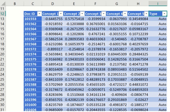
In this example, we will use the Logistic Regression Classification method to create a classification model using the Concept Document matrix on TM_LSA_CDM. Recall that this matrix includes the top twenty concepts extracted from the document collection across the top of the matrix and each document in the sample down the left. Each concept will now become a “feature” and each document will now become a “record”.
First, we’ll need to append a new column with the class that the document is currently assigned: electronics or autos. Since we sorted our documents at the beginning of the example starting with Autos, we can simply enter “Autos” into column I for Document IDs 101553 through 103096 (or cells I13:I162) and enter “Electronics” into column I for Document IDs 52434 through 53879 (or cells I163:I312). Give the column the title "Type".
First, we’ll need to partition our data into two datasets, a training dataset where the model will be “trained” and a validation dataset where the newly created model can be tested, or validated. When the model is being trained, the actual class label assignments are “shown” to the algorithm in order for it to “learn” which variables (or concepts) result in an “auto” or “electronic” assignment. When the model is being validated or tested, the known classification is only used to evaluate the performance of the algorithm. Click Partition – Standard Partition on the Text Miner ribbon to open the Standard Data Partition dialog. Select all variables in the Variables In Input Data listbox, then click > to move all to the Selected Variables listbox. Select Specify percentages Under Partitioning percentages when picking up rows randomly (at the bottom) and enter 80 for Training Set. Automatically, 20 will be entered for Validation Set.
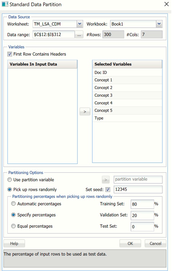
Click Finish to partition the data into two randomly selected datasets: The Training dataset containing 80% of the “records” (or documents) and the Validation dataset containing 20% of the “records”. (For more information on partitioning, please see the Standard Partitioning chapter that appears in the Analytic Solver Data Science Reference Guide.)
Now click Classify – Logistic Regression to open the Logistic Regression – Step 1 of 3 dialog. Select all 5 concents under Variables In Input Data listbox and click > to move them to the Selected Variables listbox. Doing so selects these variables as inputs to the classification method. Select Type, then click the > next to Output Variable to add this variable as the Output Variable.
Click Finish to accept all defaults and run Logistic Regression.
Select DA_ValidationScore tab and scroll down to the Validation Classification Summary, shown below.
Text Miner used the training dataset to “train” the Logistic Regression model to classify each “record” (or document) as an “autos” or “electronics” document. Afterwards, Text Miner tested the newly created Logistic Regression model on the records in the validation dataset and assigned each record (or document) a classification.
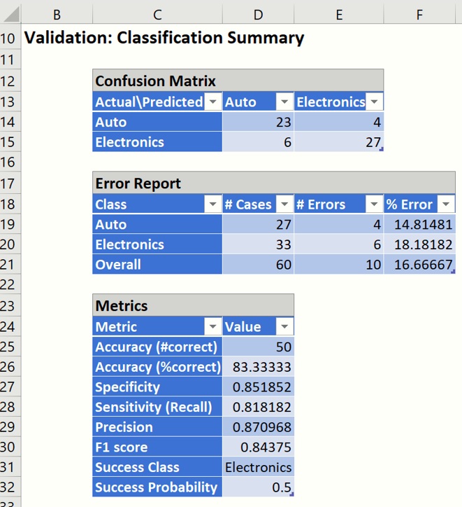
As you can see in the reports above, Logistic Regression was able to correctly classify 50 out of a total of 60 documents in the validation partition, which translates to an overall error of 16.67%, (For more information on how to read the summary report, see the Logistic Regression chapter later on in this guide.)
This concludes our example on how to use Analytic Solver Data Science’s Text Miner feature. This example has illustrated how Analytic Solver Data Science provides powerful tools for importing a collection of documents for comprehensive text preprocessing, quantitation, and concept extraction, in order to create a model that can be used to process new documents – all performed without any manual intervention. When using Text Miner in conjunction with our classification algorithms, Analytic Solver Data Science can be used to classify customer reviews as satisfied/not satisfied, distinguish between which products garnered the least negative reviews, extract the topics of articles, cluster the documents/terms, etc. The applications for Text Miner are endless!