The key property of functions of the variables that makes a problem “easy” or “hard” to solve is convexity. If all constraints in a problem are convex functions of the variables, and if the objective is convex if minimizing, or concave if maximizing, then you can be confident of finding a globally optimal solution (or determining that there is no feasible solution), even if the problem is very large.
In contrast, if any of the constraints are non-convex, or if the objective is either non-convex, concave if minimizing, or convex if maximizing, then the problem is far more difficult: You cannot be certain of finding a feasible solution even if one exists; you must either “settle for” a locally optimal solution, or else be prepared for very long solution times and rather severe limits on the size of problems you can solve to global optimality, even on the fastest computers. So it pays to understand convexity!
This property extends well beyond the scope of problems that Solver can handle; convex optimization models with hundreds of thousands or even millions of variables can be solved routinely with advanced Solvers, but there are non-convex models with hundreds of variables that have never been solved.
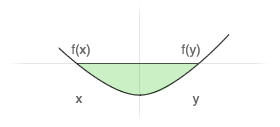
Geometrically, a function is convex if, at any two points x and y, the line drawn from x to y (called the chord from x to y) lies on or above the function – as shown in the diagram below, for a function of one variable. A function is concave if the chord from x to y lies on or below the function. This property extends to any number of ‘dimensions’ or variables, wherex = (x1, x2, …, xn) and y =( y1, y2, …, yn).

Algebraically, a function f is convex if, for any points x and y, and any t between 0 and 1, f( tx + (1-t)y ) <= tf(x) + (1-t)f(y). A function f is concave if –f is convex, i.e. if f( tx + (1-t)y ) >= tf(x) + (1-t)f(y). A linear function is both convex and concave: The chord from x to y lies on the line, and f( tx + (1-t)y ) = tf(x) + (1-t)f(y). A problem with all linear functions is the simplest example of a convex optimization problem that can be solved efficiently and reliably to very large size.
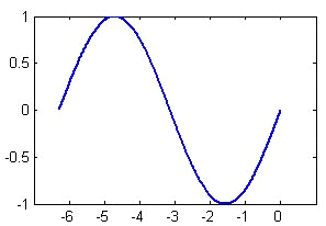
A non-convex function “curves up and down.” A familiar example is the sine function (SIN(C1) in Excel), which is pictured below.

The feasible region of an optimization problem is formed by the intersections of the constraints. The intersection of several convex constraints is always a convex region, but even one non-convex function can make the whole region non-convex – and hence make the optimization problem far more difficult to solve.
