Data collected over time is likely to show some form of random variation. "Smoothing techniques" can be used to reduce or cancel the effect of these variations. These techniques, when properly applied, will “smooth” out the random variation in the time series data to reveal any underlying trends that may exist.
Exponential smoothing is one of the more popular smoothing techniques due to its flexibility, ease in calculation and good performance. The user can select a value for the "damping constant". A large damping factor smooths out the peaks and valleys in the dataset more so then a small damping factor.
Note: Reasonable alpha values are 0.2 to 0.3. An alpha value of 0.2 will result in a 20 percent adjustment to the current forecast.
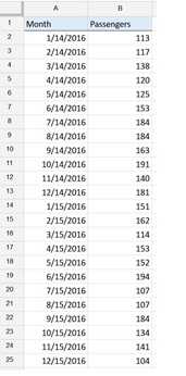
The example time series dataset below contains the monthly airline passengers in thousands for a small regional airline. Create a forecast using this historical data as input.

To generate the forecast:
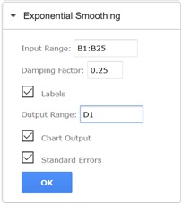
- On the XLMiner Analysis ToolPak pane, click Exponential Smoothing
- Click the Input Range field and then enter the cell range B1:B25.
- Enter a value for Damping Factor, in this example we'll use 0.25.
- Leave "Labels" selected since the first row in the data range includes the column label.
- Click the Output Range field and then select cell D1.
- Keep Chart Output selected to display the chart output in the report.
- Keep Standard Errors selected to display the standard errors in the report.
- Click OK.

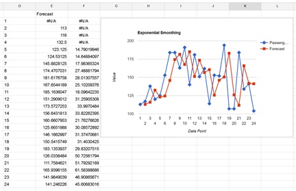
The results are below.

The results of the exponential smoothing have been inserted into cells E1:E25 while the standard errors have been displayed in cells F1:F25.
Note the N/A errors in the first cell of column E and the first four of column F are due to insufficient historical values needed to project a forecast or calculate a standard error.
