The Analytic Solver Data Science Feature Selection tool provides the ability to rank and select the most relevant variables for inclusion in a classification or prediction model. In many cases, the most accurate models (i.e., the models with the lowest misclassification or residual errors) have benefited from better feature selection, using a combination of human insights and automated methods. ASDM provides a facility to compute all of the following metrics -- described in the literature -- to provide information on which features should be included or excluded from their models.
- Correlation-based
- Pearson product-moment correlation
- Spearman rank correlation
- Kendall concordance
- Statistical/probabilistic independence metrics
- Welch's statistic
- F-statistic
- Chi-square statistic
- Information-theoretic metrics
- Mutual Information (Information Gain)
- Gain Ratio
- Other
- Cramer's V
- Fisher score
- Gini index
Only some of these metrics can be used in any given application, depending upon the characteristics of the input variables (features) and the type of problem. In a supervised setting, we can classify data science problems (as in the following) and describe the applicability of the Feature Selection metrics by the sections below.
- Rn → R: real-valued features, prediction (regression) problem
- Rn → {0,1}:: real-valued features, binary classification problem
- Rn → {1...C}: real-valued features, multi-class classification problem
- {1...C}n → Rn: nominal categorical features, prediction (regression) problem
- {1...C}n → {0, 1} nominal categorical features, binary classification problem
- {1...C}n → {1...C}: nominal categorical features, multi-class classification problem
Pearson, Spearman, and Kendall
Metrics can be applied naturally to real-valued features in a prediction (regression problem)
-------------------------------------------------------------------------------------------------------
Welch's Test
Features or the outcome variable must be discretized before applying filter to real-valued features in a prediction (regression) problem
Metrics can be applied naturally to real-valued features in a binary classification problem
-------------------------------------------------------------------------------------------------------
F-Test, Fisher, and Gini
Features or the outcome variable must be discretized before applying filter to real-valued features in a prediction (regression) problem
Metrics can be applied naturally to real-valued features in a binary classification problem
Metrics can be applied naturally to real-valued features in a multi-class classification problem
-------------------------------------------------------------------------------------------------------
Chi-squared, Mutual Info, and Gain Ratio
Features or the outcome variable must be discretized before applying filter to real-valued features in a prediction (regression) problem
Features or the outcome variable must be discretized before applying filter in a binary classification problem
Features or the outcome variable must be discretized before applying filter in a multi-class classification problem
Features or the outcome variable must be discretized before applying filter in a prediction (regression) problem with nominal categorical features
Metrics can be applied naturally to real-valued features in a binary classification problem with nominal categorical features
Metrics can be applied naturally to real-valued features in a multi-class classification problem with nominal categorical features
Depending upon the variables (features) selected and the type of problem chosen in the first dialog, various metrics are available or disabled in the second dialog.
___________________________________________________________________________________________________________________________________________________________________
Feature Selection Example
The goal of this example is: 1) to use Feature Selection as a tool for exploring relationships between features and the outcome variable; 2) reduce the dimensionality based on the Feature Selection results; and 3) evaluate the performance of a supervised learning algorithm (a classification algorithm) for different feature subsets.
This example uses the Heart Failure Clinical Records Dataset[1], which contains thirteen variables describing 299 patients experiencing heart failure. The journal article referenced here discusses how the authors analyzed the dataset to first rank the features (variables) by significance and then used the Random Trees machine learning algorithm to fit a model to the dataset. This example attempts to emulate their results.
A description of each variable contained in the dataset appears in the table below.
| Variable | Description |
|---|---|
| Age | Age of patient |
| Anaemia | Decrease of red blood cells or hemoglobin (boolean) |
| creatinine_phosphokinase | Level of the CPK enzyme in the blood (mcg/L) |
| diabetes | If the patient has diabetes (boolean) |
| ejection_fraction | Percentage of blood leaving the heart at each contraction (percentage) |
| high_blood_pressure | If the patient has hypertension (boolean) |
| platelets | Platelets in the blood (kiloplatelets/mL) |
| serum_creatinine | Level of serum creatinine in the blood (mg/dL) |
| serum_sodium | Level of serum sodium in the blood (mEq/L) |
| sex | Woman (0) or man (1) |
| smoking | If the patient smokes or not (boolean) |
| time | Follow-up period (days) |
| DEATH_EVENT | If the patient deceased during the follow-up period (boolean) |
To open the example dataset, click Help – Example Models – Forecasting/Data Science Examples – Heart Failure Clinical Records.
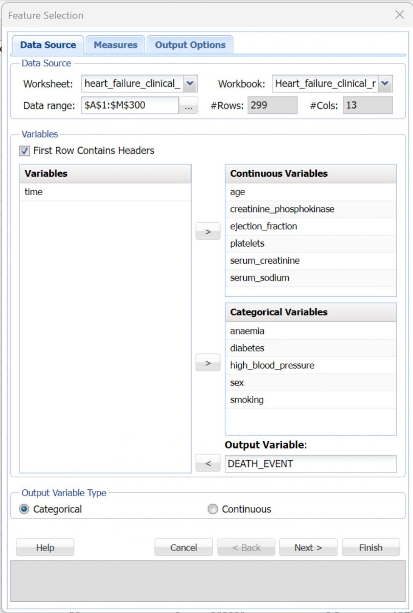
Select a cell within the data (say A2), then click Explore – Feature Selection to bring up the first dialog.
- Select all the following variables as Continuous Variables: age, creatinine_phosphokinase, ejection_fraction, platelets, serum_creatinine and serum_sodium.
- Select the following variables as Categorical Variables: anaemia, diabetes, high_blood_pressure, sex and smoking.
- Select DEATH_EVENT as the Output Variable
- Confirm that Categorical is selected for Output Variable Type. This setting denotes that the Output Variable is a categorical variable. If the number of unique values in the Output variable is greater than 10, then Continuous will be selected by default. However, at any time the User may override the default choice based on his or her own knowledge of the variable.
This analysis omits the time variable. The Feature Selection dialog should look similar to Figure 1 below.
Figure 1: Feature Selection Data Source dialog
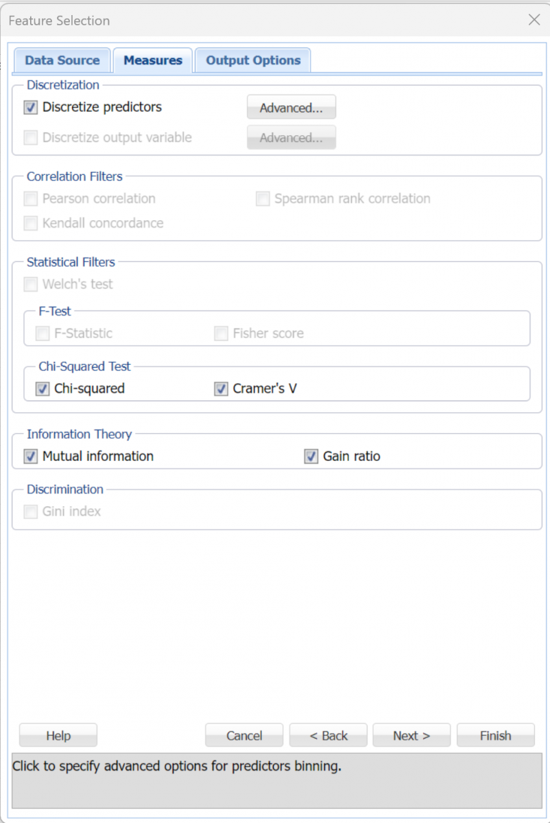
Click the Measures tab or click Next to open the Measures dialog.
Since we have continuous variables, Discretize predictors is enabled. When this option is selected, Analytic Solver Data Science will transform continuous variables into discrete, categorical data in order to be able to calculate statistics, as shown in the table in the Introduction to this chapter.
This dataset contains both continuous (or real-valued) features and categorical features which puts this dataset into the following category.
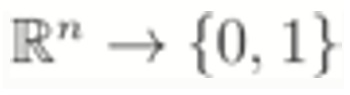 : real-valued features, binary classification problem
As a result, if interested in evaluating the relevance of features according to the Chi-Squared Test or measures available in the Information Theory group (Mutual Information and Gain ratio), the variables must first be discretized.
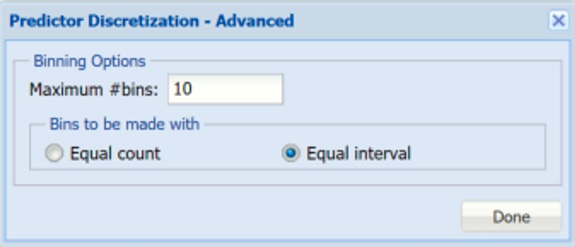
Select Discretize predictors, then click Advanced. Leave the defaults of 10 for Maximum # bins and Equal Interval for Bins to be made with. Analytic Solver Data Science will create 10 bins and will assign records to the bins based on if the variable’s value falls in the interval of the bin. This will be performed for each of the Continuous Variables.
Figure 2: Predictor Discretization - Advanced
Note: Discretize output variable is disabled because our output variable, DEATH_EVENT, is already a categorical nominal variable. If we had no Continuous Variables and all Categorical Variables, Discretize predictors would be disabled.
Select Chi-squared and Cramer’s V under Chi-Squared Test. The Chi-squared test statistic is used to assess the statistical independence of two events. When applied to Feature Selection, it is used as a test of independence to assess whether the assigned class is independent of a particular variable. The minimum value for this statistic is 0. The higher the Chi-Squared statistic, the more independent the variable.
Cramer’s V is a variation of the Chi-Squared statistic that also measures the association between two discrete nominal variables. This statistic ranges from 0 to 1 with 0 indicating no association between the two variables and 1 indicating complete association (the two variables are equal).
Select Mutual information and Gain ratio within the Information Theory frame. Mutual information is the degree of a variables’ mutual dependence or the amount of uncertainty in variable 1 that can be reduced by incorporating knowledge about variable 2. Mutual Information is non-negative and is equal to zero if the two variables are statistically independent. Also, it is always less than the entropy (amount of information contained) in each individual variable.
The Gain Ratio, ranging from 0 and 1, is defined as the mutual information (or information gain) normalized by the feature entropy. This normalization helps address the problem of overemphasizing features with many values but the normalization results in an overestimate of the relevance of features with low entropy. It is a good practice to consider both mutual information and gain ratio for deciding on feature rankings. The larger the gain ratio, the larger the evidence for the feature to be relevant in a classification model.
For more information on the remaining options on this dialog, see the Using Feature Selection below.
Figure 3: Feature Selection Measures dialog
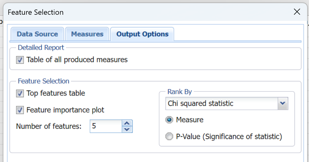
Click the Output Options tab or click Next to open the Output Options dialog. Table of all produced measures is selected by default. When this option is selected, Analytic Solver Data Science will produce a report containing all measures selected on the Measures tab.
Top Features table is selected by default. This option produces a report containing only top variables as indicated by the Number of features edit box.
Select Feature importance plot. This option produces a graphical representation of variable importance based on the measure selected in the Rank By drop down menu.
Enter 5 for Number of features. Analytic Solver Data Science will display the top 5 most important or most relevant features (variables) as ranked by the statistic displayed in the Rank By drop down menu.
Keep Chi squared statistic selected for the Rank By option. Analytic Solver Data Science will display all measures and rank them by the statistic chosen in this drop down menu.
Figure 4: Feature Selection Output Options dialog
Click Finish.
Two worksheets are inserted to the right of the heart_failure_clinical_records worksheet: FS_Output and FS_Top_Features.
Click the FS_Top_Features tab.
Note: In the Data Science Cloud app, click the Charts icon on the Ribbon to open the Charts dialog, then select FS_Top_Features for Worksheet and Feature Importance Chart for Chart.
The Feature Importance Plot ranks the variables by most important or relevant according to the selected measure. In this example, we see that the ejection_fraction, serum_creatinine, age, serum_sodium and creatinine_phosphokinase are the top five most important or relevant variables according to the Chi-Squared statistic. It’s beneficial to examine the Feature Selection Importance Plot in order to quickly identify the largest drops or “elbows” in feature relevancy (importance) and select the optimal number of variables for a given classification or regression model.
Note: We could have limited the number of variables displayed on the plot to a specified number of variables (or features) by selecting Number of features and then specifying the number of desired variables. This is useful when the number of input variables is large or we are particularly interested in a specific number of highly – ranked features.
Run your mouse over each bar in the graph to see the Variable name and Importance factor, in this case Chi-Square, in the top of the dialog.
Click the X in the upper right hand corner to close the dialog, then click FS_Output tab to open the Feature Selection report.
Figure 5: Feature Selection: Statistics
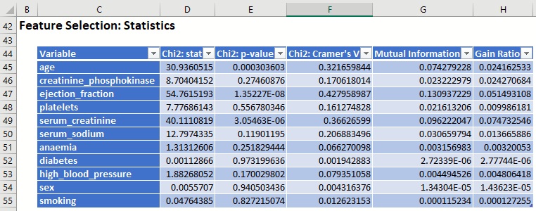
The Detailed Feature Selection Report displays each computed metric selected on the Measures tab: Chi-squared statistic, Chi-squared P-Value, Cramer’s V, Mutual Information, and Gain Ratio.
Chi2: Statistic and p-value
Click the down arrow next to Chi2: p-value to sort the table according to this statistic going from smallest p-value to largest.
Figure 6: Statistics sorted by Chi2:p-value
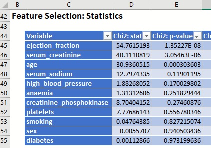
According to the Chi-squared test, ejection_fraction, serum_creatinine and age are the 3 most relevant variables for predicting the outcome of a patient in heart failure.
Chi2: Cramer's V
Recall that the Cramer's V statistic ranges from 0 to 1 with 0 indicating no association between the two variables and 1 indicating complete association (the two variables are equal). Sort the Cramer's V statistic from largest to smallest.
Figure 7: Chi2: Cramer's V Statistic
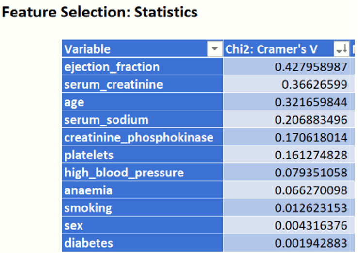
Again, this statistics ranks the same four variables, ejection_fraction, serum_creatinine, age and serum_sodium, as the Chi2 statistic.
Mutual Information
Sort the Mutual Information column by largest to smallest value. This statistic measures how much information the presence/absence of a term contributes to making the correct classification decision.[2] The closer the value to 1, the more contribution the feature provides.
Figure 8: Mutual Information Statistic

When compared to the Chi2 and Cramer's V statistic, the top four most significant variables calculated for Mututal Information are the same: ejection_fraction, serum_creatinine, age, and serum_sodium.
Gain Ratio
Finally, sort the Gain Ratio from largest to smallest. (Recall that the larger the gain ratio value, the larger the evidence for the feature to be relevant in the classification model.)
Figure 9: Gain Ratio
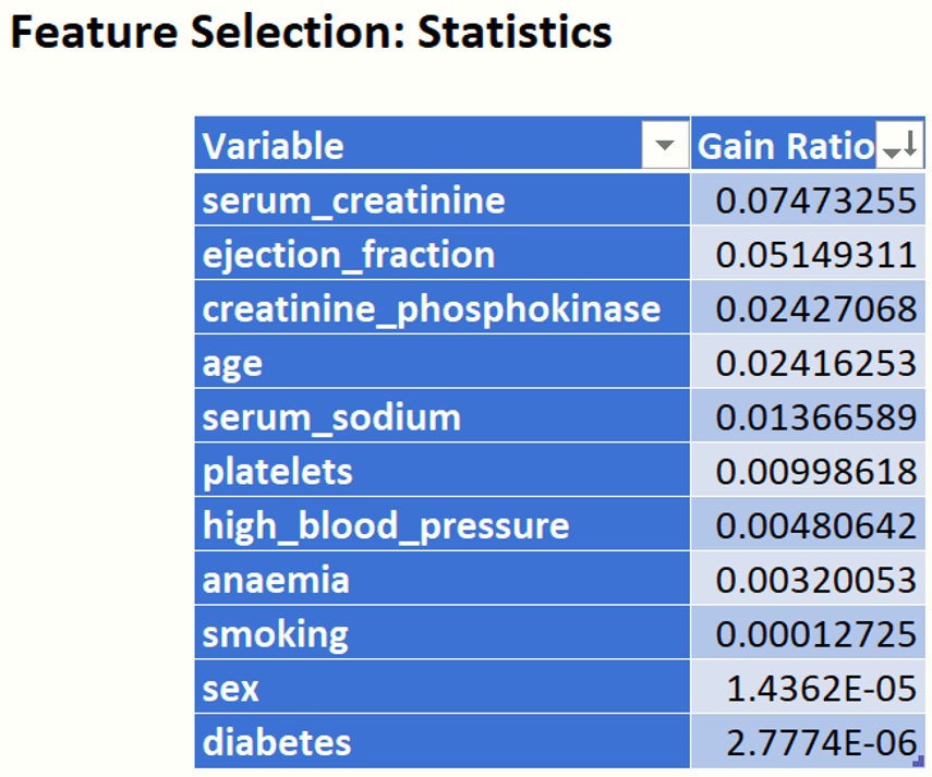
While this statistic's rankings differ from the first 4 statistic's rankings, ejection_fraction, age and serum_creatinine are still ranked in the top four positions.
The Feature Selection tool has allowed us to quickly explore and learn about our data. We now have a pretty good idea of which variables are the most relevant or most important to our classification or prediction model, how our variables relate to each other and to the output variable, and which data attributes would be worth extra time and money in future data collection. Interestingly, for this example, most of our ranking statistics have agreed (mostly) on the most important or relevant features with strong evidence. We computed and examined various metrics and statistics and for some (where p-values can be computed) we’ve seen a statistical evidence that the test of interest succeeded with definitive conclusion. In this example, we’ve observed that several variable (or features) were consistently ranked in the top 3-4 most important variables by most of the measures produced by Analytic Solver Data Science’s Feature Selection tool. However, this will not always be the case. On some datasets you will find that the ranking statistics and metrics compete on rankings. In cases such as these, further analysis may be required.
Fitting the Model
See the Analytic Solver User Guide for an extension of this example which fits a model to the heart_failure dataset using the top variables found by Feature Selection and compares that model to a model fit using all variables in the dataset.
[1] Davide Chicco, Giuseppe Jurman: Machine learning can predict survival of patients with heart failure from serum creatinine and ejection fraction alone. BMC Medical Informatics and Decision Making 20, 16 (2020). (link)
[2] https://nlp.stanford.edu/IR-book/html/htmledition/mutual-information-1.html