Using Psi Functions to Score Data
Analytic Solver Data Science utilizes XML PMML format to store the supported models and use them for “scoring” (classifying, predicting, forecasting, transforming) new data using four new generic scoring functions: PsiPredict(), PsiForecast(), PsiTransform() and PsiPosteriors(). PsiPredict() and PsiForecast() provide previously available functionality plus new additional functionality such as storing and scoring ensemble models with any available weak learner and computing the fitted values for new time series data. PsiTransform() and PsiPosteriors() provide new functionality and the availability of new models for storing or scoring.
| Psi Scoring Function | Description |
|---|---|
| PsiPredict() | Predicts the target for input data using a Classification or Regression model and computes the fitted values for a Time Series model stored in PMML format. |
| PsiForecast() | Computes the forecasts for the input data using a Time Series model stored in PMML format. |
| PsiPosteriors() | Computes the posterior probabilities for the input data using a Classification model stored in PMML format. |
| PsiTransform() | Transforms the input data using a Transformation model stored in PMML format. |
It’s possible to score data with a prediction or classification method or perform a time series forecast manually (without the need to click the Score icon on the ribbon) by entering a Psi Solver function into an Excel cell as an array.
Scoring Data Using Psi Functions
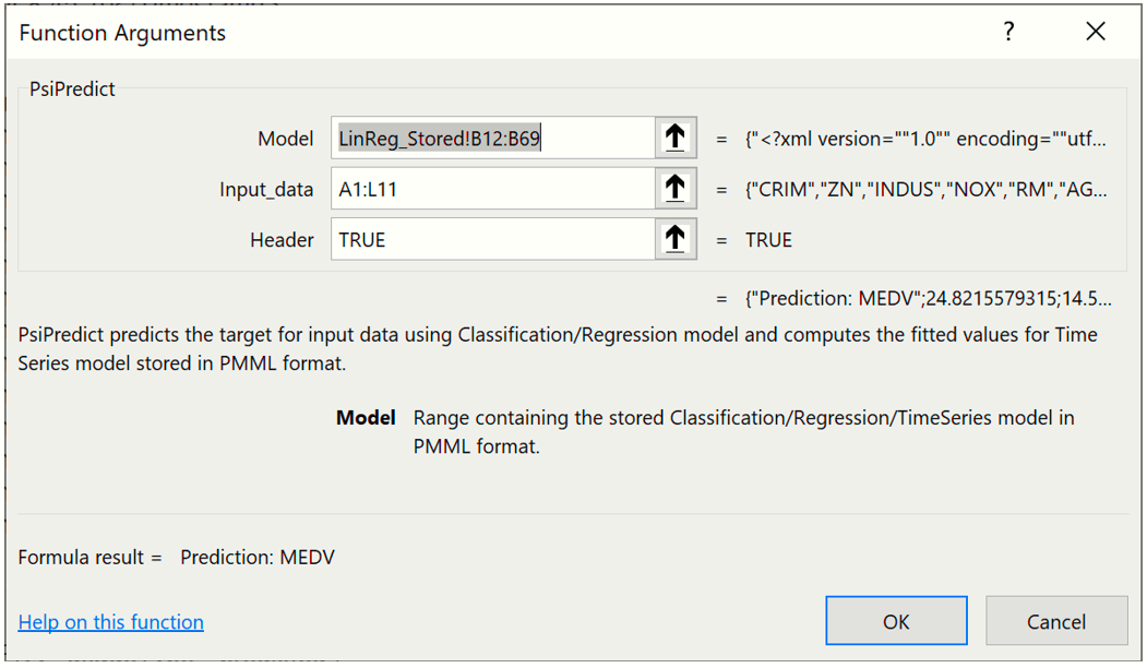
Using the example above, click over to the PsiPredict worksheet and select a blank cell on the worksheet. Enter "=PsiPredict(LinReg_Stored!B12:B69,'New Data'!A1:L11)". The formula result will "spill" into the cells below.
Note: If using a version of Excel that does not support Dynamic Arrays, select cells N1:N11, enter the formula and press SHIFT + CTRL + ENTER to enter the formula as an array into all 10 cells (N2:N11).
The first argument, LinReg_Stored!B12:B69, is the range of cells used by Analytic Solver Data Science to store the linear regression model on the LinReg_Stored worksheet. Clearly this data range will change as the classification or prediction method changes and as the number of features included in the dataset changes.
The second argument, New Data!A1:L11, is the range containing the new data on the New Data worksheet. The new data must contain at least one row of data containing the same number of features (or columns) as the data used to create the model. In this example, we included 12 features in the linear regression model: CRIM, ZN, INDUS, NOX, RM, AGE, DIS, RAD, TAX, PTRATIO, B & LSTAT. As a result, our new data also containes these same 12 features. We could have performed this prediction on only one row of new data, NewData!A2:L2, but choose to use all 10 rows.
Note: If there are new or missing features in the new dataset, the Psi Data Science function will return #VALUE.
It’s also possible to enter this formula using the Insert Function dialog by clicking Formulas – Insert Function, select PSI Data Science for Category, then PsiPredictMLR.
Note: The Insert Function dialog is not supported when using Data Science Cloud. To use this function or any other Psi function, simply type the function directly into the cell.
The scoring results are shown in the screenshot below in the N column.
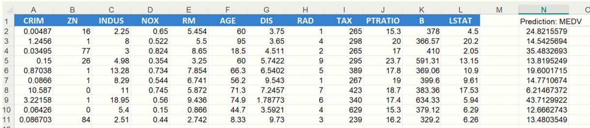
The PsiPredict() function is interactive meaning that if a variable value is changed, for example the first LSTAT value in cell L2 changes from 4.5 to 9.5, the Predicted Value in cell N2 will immediately update to reflect a new predicted value.
The remaining PSI Data Science functions can be used in the same way using models from their respective stored model sheets. See below for specifications for PsiPredict(), PsiPosteriors() and PsiTransform(). See the section below for information on PsiForecast().
PsiPredict()
PsiPredict(Model, Input_Data, [Header])
Predicts the response, target, output or dependent variable for Input_Data whether it is continuous (Regression) or categorical (Classification) when the model is stored in PMML format. In addition, this function also computes the fitted values for a Time Series model when the model is stored in PMML format.
Model: Range containing the stored Classification, Regression or TimeSeries model in PMML format.
Input_Data: Range containing the new data for computing predictions. Range must contain a header row with column names and at least one row of data containing the exact same features (or columns) as the data used to create the model.
Header: If True, a heading will be inserted above the forecasted values. If omitted or false, a heading will not appear.
The contents of the Dynamic Array will "spill" down the column. If a nonblank cell is "blocking" the contents of the Dynamic Array, PsiForecast() will return #SPILL until such time as the blockage is removed. Use the optional numForecasts argument to specify the number of forecasts in the Dynamic Array. If not present, one forecast will be returned.
Output: A single column containing the header (if the header argument is set to TRUE) and predicted/fitted values for each record in Input_Data.
To know if the result of the prediction is continuous or categorical, you must know what kind of model you are passing as an argument to the scoring function – if you previously fitted the classification model and are now predicting the new feature vectors, you should expect to get the compatible categorical response. On the other hand, you should expect the continuous response from the new data prediction when using a fitted regression model. In previous versions, the user was expected to know the exact type model, such as Mulitple Linear Regression or Discriminant Analysis, to know what kind of output will be produced, whereas in V2017 and later, it is sufficient to know whether you’re pointing to a classification or regression model in order to determine the type of the response. Note: If the user intends to use an “unknown” model for scoring, the stored worksheets contain the complete information about the model including several clear indications of the model type and data dictionaries with the types of features and response.
In addition, PsiPredict() can compute the fitted values for the new time series based on the provided Time Series model. Unlike future-looking forecasting, provided by PsiForecast(), PsiPredict() computes a model prediction for each observation in the provided new time series.
Supported Models:
- Classification:
- Linear Discriminant Analysis
- Logistic Regression
- K-Nearest Neighbors
- Classification Tree
- Naïve Bayes
- Neural Network
- Random Trees
- Bagging (with any supported weak learner)
- Boosting (with any supported weak learner)
- Regression:
- Logistic Regression
- K-Nearest Neighbors
- Neural Network
- Bagging (with any supported weak learner)
- Boosting (with any supported weak learner)
- Time Series (fitted values)
- ARIMA
- Exponential Smoothing
- Double Exponential Smoothing
- Holt-Winters Smoothing
| Prediction/Classification/Time Series Algorithem | Stored Model Sheet |
|---|---|
| Linear Discriminant Analysis Classification | DA_Stored |
| Logistic Regression Classification | LogReg_Stored |
| k-Nearest Neighbors Classification | KNNC_Stored |
| Classification Trees | CT_Stored |
| Naive Bayes Classification | NB_Stored |
| Neural Networks Classification | NNC_Stored |
| Ensemble Methods for Classification | CBoosting_Stored |
| Linear Regression | CBagging_Stored |
| k-Nearest Neighbors Regression | CRandTrees_Stored |
| Regression Tree | RT_Stored |
| Neural Network Regression | NNP_Stored |
| Ensemble Methods for Regression |
RBoosting_Stored RBagging_Stored RRandTrees_Stored |
| ARIMA | ARIMA_Stored |
| Exponential Smoothing | Expo_Stored |
| Double Exponential Smoothing | DoubleExpo_Stored |
| Moving Average Smoothing | MovingAvg_Stored |
| Holt Winters Smoothing |
MultHoltWinters_Stored AddHoltWinters_Stored NoTrendHoltWinters_Stored |
Classification: PsiClassifyLR, PsiClassifyDA, PsiClassifyCT, PsiClassifyNB, PsiClassifyNN, PsiClassifyCTEnsemble, PsiClassifyNNEnsemble
Regression: PsiPredictMLR, PsiPredictRT, PsiPredictNN, PsiPredictNNEnsemble, PsiPredictRTEnsemble
PsiPosteriors()
PsiPosteriors(Model, Input_Data, [Header])
Computes the posterior probabilities for Input_Data using a Classification model stored in PMML format.
Model: Range containing the stored Classification model in PMML format.
Input_Data: Range containing the new data for computing posterior probabilities. Range must contain a header with column names and at least one row of data containing the exact same features (or columns) as the data used to create the model.
Header: If True, a heading is inserted in the output above the forecasted values. If False or omitted, a heading is not inserted into the output.
The contents of the Dynamic Array will "spill" down the column. If a nonblank cell is "blocking" the contents of the Dynamic Array, PsiForecast() will return #SPILL until such time as the blockage is removed. Use the optional numForecasts argument to specify the number of forecasts in the Dynamic Array. If not present, one forecast will be returned.
Output: Multiple columns containing a header with class labels and estimated posterior probabilities for each class label for all records in Input_Data.
Supported Models:
- Classification:
- Linear Discriminant Analysis
- Logistic Regression
- K-Nearest Neighbors
- Classification Tree
- Naïve Bayes
- Neural Network
- Random Trees
- Bagging (with any supported weak learner)
- Boosting (with any supported weak learner)
Previous related Psi Scoring functions: N/A
| Classification Algorithm | Stored Model Sheet |
|---|---|
| Linear Discriminant Analysis Classification | DA_Stored |
| Logistic Regression Classification | LogReg_Stored |
| k-Nearest Neighbors Classification | KNNC_Stored |
| Classification Trees | CT_Stored |
| Naive Bayes Classification | NB_Stored |
| Neural Networks Classification | NNC_Stored |
| Ensemble Methods for Classification |
CBoosting_Stored CBagging_Stored CRandTress_Stored |
PsiTransform()
PsiTransform(Model, Input_Data, [Header])
Transforms the Input_Data using a Transformation model stored in PMML format.
Model: Range containing the stored Transformation model in PMML format.
Input_Data: Range containing the new data for transformation. Range must contain a header with column names and at least one row of data containing the exact same features (or columns) as the data used to create the model.
Header: If True, a heading is inserted above the forecasted values. If False or omitted, a heading is not inserted.
The contents of the Dynamic Array will "spill" down the column. If a nonblank cell is "blocking" the contents of the Dynamic Array, PsiForecast() will return #SPILL until such time as the blockage is removed. Use the optional numForecasts argument to specify the number of forecasts in the Dynamic Array. If not present, one forecast will be returned.
Output: One or multiple columns containing a header and transformed data.
Supported Models:
- Transformation:
- Rescaling
- Text Mining
- TF-IDF Vectorization (input data – text variable with the corpus of documents)
- LSA Concept Extraction (input data – term-document matrix, where columns represent terms and rows represent documents)
Previous related Psi Scoring functions: N/A
| Algorithm | Stored Model Sheet |
|---|---|
| Rescaling | Rescaling_Stored |
| Text Mining |
TFIDF_Stored LSA_Stored |
Time Series Forecasting
Starting with version 2014-R2, Analytic Solver Data Science includes the ability to forecast a future point in a time series in one of your spreadsheet formulas (without using the Score button on the Ribbon) using a PsiForecast() function in conjunction with a model created using ARIMA or one of our smoothing methods (Exponential, Double Exponential, Moving Average, or Holt Winters).
PsiForecast() is similar to the previous PSIForecastXXX functions supported in V2014, 2015, and 2016: it will compute future-looking forecasts based on the fitted model, using the provided new time series observations as initial points. The result of PsiForecast() can be deterministic, if the Simulate argument is FALSE, or non-deterministic, if the Simulate argument is TRUE– in which case the forecasts are adjusted with random normally distributed errors, defined by the forecasts’ statistics.
Open the Airpass.xlsx example dataset by clicking Help – Examples on the Data Science ribbon, then clicking Forecasting/Data Science Examples. This example dataset includes International Airline Passenger Information by month for years 1949 – 1960. Since the number of airline passengers increases during certain times of the year, for example Spring, Summer, and in the month of December, we can say that this dataset includes “seasonality”.
First, we will partition this dataset into two datasets: a training dataset and a validation dataset. We’ll use the training dataset to create the ARIMA model and then we’ll apply the model to the validation dataset to forecast six future data points, or one half year of data.
Click Partition in the Time Series section of the Data Science ribbon to open the Time Series Partition Data dialog. Select Passengers for the Variables in the Partition Data and Month for the Time Variable.
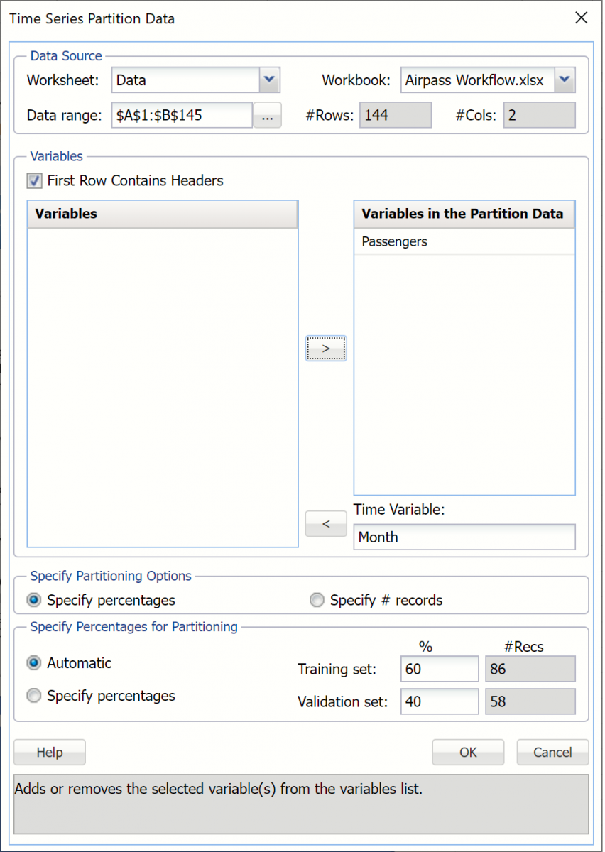
Click OK to accept the defaults for Specify Partitioning Options and Specify Percentages for Partitioning. Recall that when a time series dataset is partitioned, the dataset is partitioned sequentially. Therefore, 60% or the first 86 records, will be assigned to the training dataset and the remaining 40%, or 58 records, will be assigned to the validation dataset. (For more information on partitioning a time series dataset, see Exploring a Time Series Dataset.)
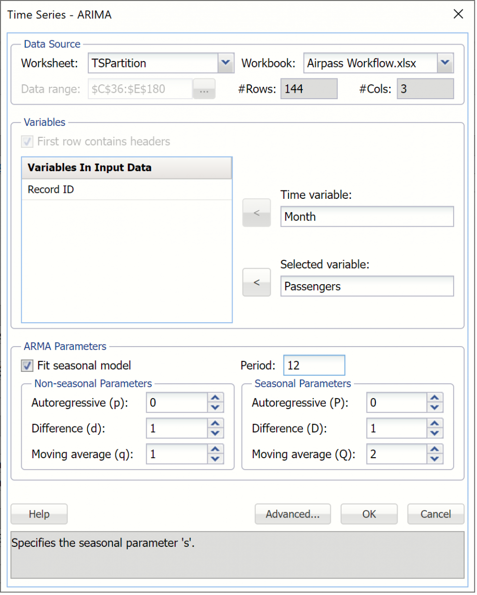
The TSPartition worksheet will be inserted into the Model tab of the Analytic Solver task pane under Transformations – Time Series Partition. Recall the steps needed to produce the forecast. Click ARIMA -- ARIMA to open the ARIMA dialog. Month has been pre selected as the Time variable. Select Passengers as the Selected variable.
This example will use a SARIMA model, or Seasonal Autoregressive Integrated Moving Average model, to predict the next six datapoints in the dataset. A seasonal ARIMA model requires 7 parameters, 3 nonseasonal (autoregressive (p), integrated (d), and moving average (q)), 3 seasonal (autoregressive (P), integrated (D), and moving average (Q)), and period. Each parameter must be a non-negative integer.
Selecting appropriate values for p, d, q, P, D, Q and period is beyond the scope of this User Guide. Consequently, this example will use a well documented SARIMA model with parameters p = 0, d = 1, q = 1, P = 0, D = 1, Q = 2 and period (P) = 12. Please refer to the classic time series analysis text Time Series Analysis: Forecasting and Control written by George Box and Gwilym Jenkins for more information on parameter selection.
Select Fit seasonal model and enter 12 for Period since it takes a full 12 months for the seasonal pattern to repeat. Set the Non-seasonal Parameters as Autoregressive (p) = 0, Difference (d) = 1, Moving Average (q) = 1 and the Seasonal Parameters as Autoregressive (P) = 0, Difference (D) = 1, and Moving Average (Q) = 2.
Click OK to create the SARIMA model.
ARIMA_Output will be inserted into the Model tab of the task pane under Reports – ARIMA. This output contains the Training Error Measures and Fitted Model Statistics. ARIMA_Stored contains the stored model parameters.
Now we’ll use this ARIMA model to predict new data points in the validation dataset using the PsiForecast() function. When entered, this function will forecast seven different future points in the dataset. (Note: The first forecasted point will be more accurate than the second, the second forecasted point more accurate than the third and so on.) The PsiForecast() function will be interactive in the sense that if any of the input values (values passed in the 2nd argument) change, the forecast will be recomputed.
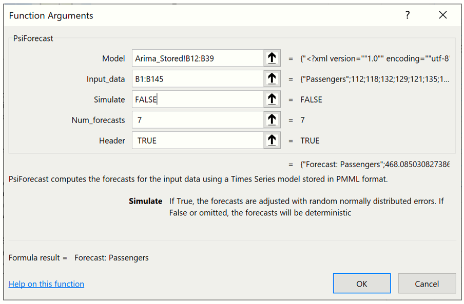
The PsiForecastARIMA function takes five arguments but two are optional: Model, Input Data, Simulate, Num_forecasts, and Header. Select a blank cell on the Data worksheet and enter =PsiForecast(.
Note: If using a version of Excel that does not support Dynamic Arrays, highlight cells B146:B152, then enter =PsiForecast(.
The first argument, Model, is the range of cells used by Analytic Solver Data Science to store the ARIMA model on the ARIMA_Stored worksheet. This data range will change as the forecast method changes. Select or enter ARIMA_Stored!B12:B39, for this argument.
The second argument, Input_Data, is the range containing the initial starting points from the validation data set. The minimum number of initial points that should be specified for a seasonal ARIMA model is the larger of p + d + s * (P + D) and q + s * Q. In this example, p + d + s * (P + D) is equal to 13 (0 + 1 + 12 * (0 + 1) and q + s * Q is equal to 13 (1 + 12 * 1), therefore the minimum number of initial starting points required is 13 (MAX (13, 13)). If you provide fewer than the minimum required number of starting points, PsiForecast() will return a column of zeros. (See the table below for the minimum number of initial starting points required by each Forecasting method included in Analytic Solver Data Science.) The maximum number of starting points is the number of points in the validation dataset. All points supplied in the second argument will be used in the forecast. Select or enter Data!B1:B145, for this argument.
Pass True or False for the third argument. Passing False will result in a static forecast that will only update if a cell passed in the 2nd argument is changed. If True is passed for this argument, a random error will be included in the forecasted points. See the Time Series Simulation example in the next help topic for more information on passing True for this argument. In this case, Pass False) for this argument.
Pass "7" for the next argument, number of forecasts.
Pass "True" for header to display a heading title at the top of the results.
Your formula should now be =PsiForecast(ARIMA_Stored!B12:B39,Data!B1:B145, False, 7, True).
Note: If using a version of Excel that does not support Dynamic Arrays, press CTRL + SHIFT + ENTER to enter this formula as an array in all seven cells (B146:B152).
It’s also possible to enter this formula using the Insert Function dialog by clicking Formulas – Insert Function, select PSI Data Science for Category, then PsiForecastARIMA.
The results from this function are displayed below.
Notice that the formula is entered into cell B146 and the contents of the PsiForecast() Dynamic Array "spill" down into cells B147:B152.
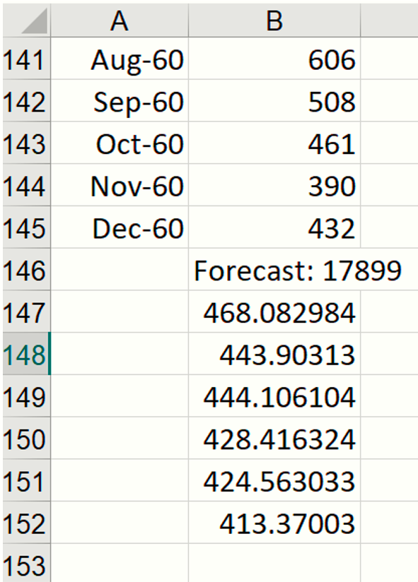
If any values change in the ranges ARIMA_Stored!B12:B38 or Data!B2:B145, the forecast will be recomputed; but if the input argument values stay the same, the PsiForecast() function will always return the same forecast values. As mentioned above, the first forecasted value is the most accurate predicted point. Accuracy declines as the number of forecasted points increases.
See the section below for specifications on PsiForecast().
PsiForecast()
PsiForecast(Model, Input_Data, [Simulate], [Num_Forecasts], [Header])
Computes the forecasts for Input_Data using a Time Series model stored in PMML format.
Model: Range containing the stored Times Series model in PMML format.
Input_Data: Range containing the new Time Series data for computing the forecasts. Range must contain a header with the time series name and a sufficient number of records for the forecasting with a given model.
Simulate: If True, the forecasts are adjusted with random normally distributed errors. If False or omitted, the forecasts will be deterministic.
Num_Forecasts: Enter the number of desired forecasts.
Header: If True, a heading will be inserted above the forecasted results. If False or omitted, a heading will not be included in the result.
Output: A single column containing the header, if used, and forecasts for input time series. The number of produced forecasts is determined by the number of selected cells in the array-formula entry.
Supported Models:
- Arima
- Exponential Smoothing
- Double Exponential Smoothing
- Holt Winters Smoothing
Previous related Psi Scoring functions: PsiForecastARIMA, PsiForecastExp, PsiForecastDoubleExp, PsiForecastMovingAvg, PsiForecastHoltWinters
Time Series Simulation
Analytic Solver Data Science includes the ability to perform a time series simulation, where future points in a time series are forecast on each Monte Carlo trial, using a model created via ARIMA or one of our smoothing methods (Exponential, Double Exponential, Moving Average, or Holt Winters).
To run a time series simulation, we must pass “True” as the third argument to PsiForecast(). When the third argument is set to True, Analytic Solver will add a random (positive or negative) “epsilon” value to each forecasted point. Each time a simulation is run, 1000 trial “epsilon” values are generated using the PsiNormal distribution with parameters mean and standard deviation computed by the PsiForecast() function. You can view the output of this simulation in the same way as you would view “normal” simulation results in Analytic Solver Comprehensive, Analytic Solver Simulation or Analytic Solver Upgrade, simply by creating a PsiOutput() function and then double clicking the Output cell to view the Simulation Results dialog.
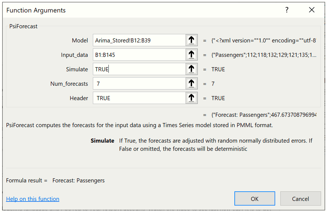
Select a blank cell, or Data!C146:C152 if using a version of Excel that does not support Dynamic Arrays, then click Formulas – Insert Function to display the Function Argument dialog.
As discussed previously, the first argument, ARIMA_Stored!B12:B38, is the range of cells used by Analytic Solver to store the ARIMA model on the ARIMA_Stored worksheet. This data range will change as the forecast method changes.
For the second argument the range containing the initial points in the series must be greater than the minimum number of initial points for a static forecast. For a seasonal ARIMA model when Simulate = True, the minimum number of initial points must be greater than Max((p + d + s * (P + D), (q + s * Q). In this example, p + d + s * (P + D) is equal to 13 (0 + 1 + 12 * (0 + 1) and q + s * Q is equal to 13 (1 + 12 * 1), therefore the minimum number of initial starting points required is 13 (Minimum #Initial Points > MAX (13, 13)). However, when PsiForecastARIMA() is called with Simulate = True, it is recommended to add an additional number of datapoints, equal to the #Periods, to the minimum number required. In this instance the number of initial points will be 25: 13 (minimum # of points) + 12 (# of points for Period in the Time Series - ARIMA dialog). If you provide fewer than the minimum required number of starting points (13 in this example) PsiForecastARIMA() will return #VALUE. (See the table below for the minimum number of initial starting points required by each forecast method in Analytic Solver.) All points supplied in the second argument will be used in the forecast. Select or enter Data!B1:B145, for this argument.
Passing TRUE for the third argument indicates to Analytic Solver Data Science that you plan to use this function call in a Monte Carlo simulation, so it should add a random epsilon value (different on each Monte Carlo trial) to each forecasted point.
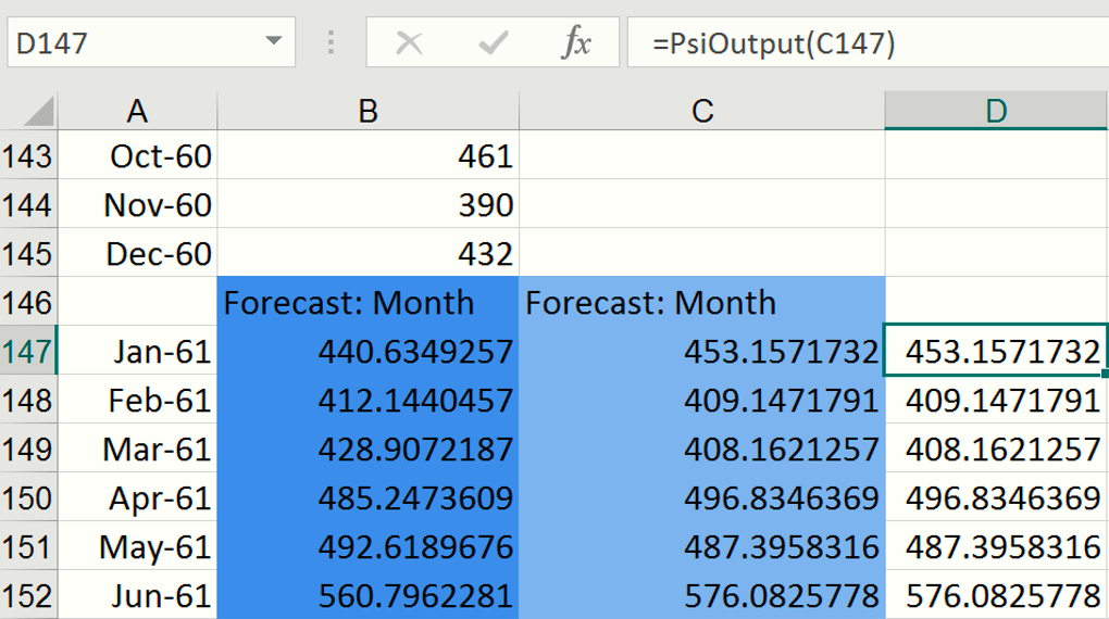
This formula is entered into cell C146 and the contents of the PsiForecast() Dynamic Array "spills" down into cells C147:C152. Note: If versions of Excel that do not support Dynamic Arrays, the formula must be entered as an Excel array.
To view the results of the simulation including frequency and sensitivity charts, statistics, and percentiles for the full range of trial values in any version of Excel, we must first create an output cell. Select cell B147, then click Analytic Solver – Results – Referred Cell. Select cell D147 (or any blank cell on the spreadsheet) to enter the PsiOutput formula. Copy this formula from cell D147 down to cell D152. Therefore D147 = PsiOutput(C147), D148 = PsiOutput(C148), and so on.
Click the down arrow on the Simulate icon and select Run Once. Instantly, Analytic Solver will perform a simulation with 1,000 Monte Carlo simulation trials (the default number). Since this is the first time a simulation has been performed, the following dialog opens. Subsequent simulations will not produce this report. However, it is possible to reopen the individual frequency charts by double clicking each of the output cells (B147:B152).
Important Note: For Users who are familiar with simulation models in Analytic Solver Simulation, you’ll notice that the time series simulation model that we just created now includes 6 uncertain functions, B147:B152, which are the cells containing our PsiForecast() functions. For more information on simulation with Analytic Solver, please see the Analytic Solver User Guide chapter, “Examples: Simulation and Risk Analysis”.
PsiForecast() is not recognized as an uncertain function in the Cloud apps. If the simulation argument is set to "True", Analytic Solver App will generate a single random point around the forecast.
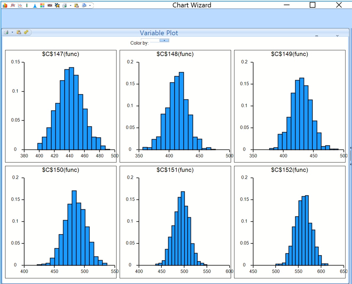
This dialog displays frequency charts for each of the six cells containing the forecasted data points. Double click the chart for cell C147 (top left) to open the Simulation Results dialog for the PsiForecast() function in cell C147. From here you can view frequency and sensitivity charts, statistics and percentiles for each forecasted point.
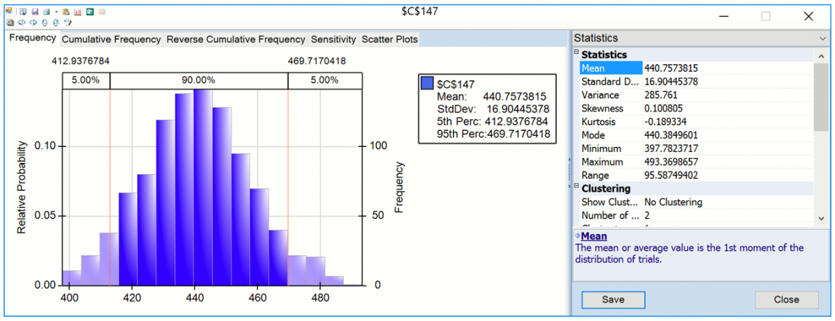
The frequency chart displays the distribution of all 1000 trial values for cell C147 with and observed mean 440.76 and standard deviation of 16.90 shown in the Chart Statistics. Select Simulate – Run Once a few more times (or click the green “play” button on the Solver Pane Model tab). Each time you do, another 1,000 Monte Carlo trials are run, and a slightly different mean will be displayed.
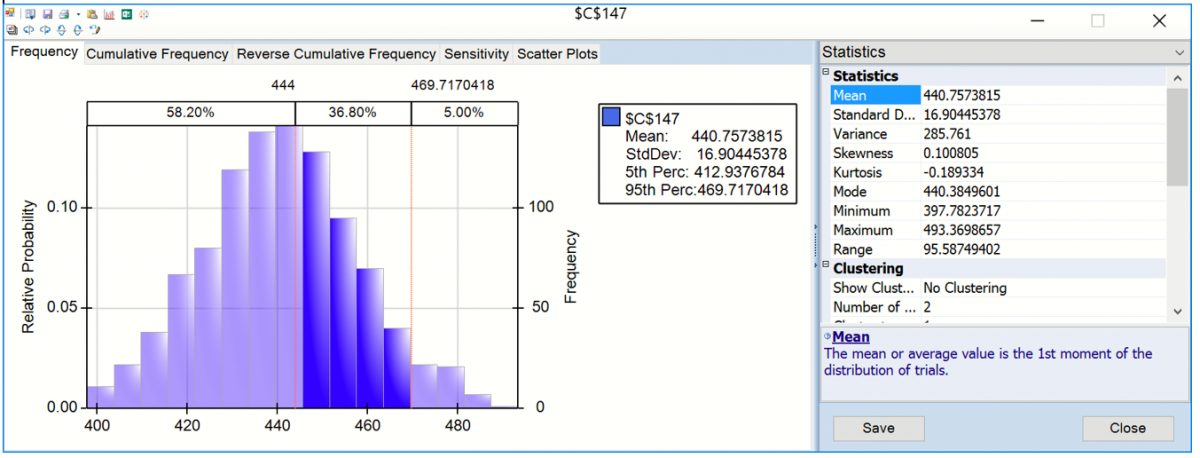
Enter 444 for the Lower Cutoff in the Chart Statistics section of the right panel, A vertical bar appears over the Frequency chart to display the frequency with which the forecasted value was greater than this value during the simulation. You can use this as an estimate of the probability that the actual value will be less than the forecasted value. In this case there was a 58.20% chance that the number of international airline passengers would be less than 444,000 in January 1961 and a 41.80% chance that the number of passengers would be greater than 444,000.
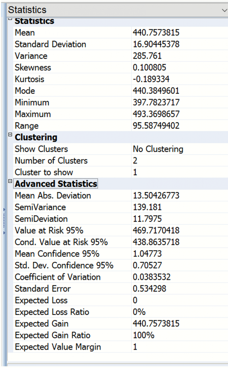
Looking to the right, you’ll find the Statistics pane, which includes summary statistics for the full range of forecasted outcomes. We can see that the minimum forecasted value during this simulation was 397.78, and the maximum forecasted value was 493.37. Value at Risk 95% shows that 95% of the time, the number of international airline passengers was 469.72 or less in January 1961, in this simulation. The Conditional Value at Risk 95% value indicates that the average number of passengers we would have seen (up to the 95% percentile) was 438.86. For more information on Analytic Solver’s full range of features, see the Analytic Solver User Guide chapter, “Examples: Simulation and Risk Analysis”.
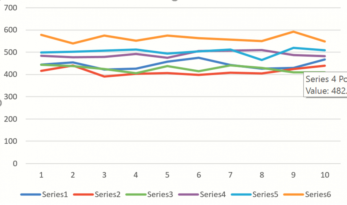
Select cells E147 and then enter the formula, =PsiData(C147), then press CTRL + SHIFT + ENTER to array enter the formula into all 10 cells. Repeat the same steps to array enter “=PsiData(C148)” in cells F147:F156, “=PsiData(C149)” in cells G147:G156, “=PsiData(C150)” in cells H147:H156, “PsiData(C151)” in cells I147:I156, and “=PsiData(C152)” in cells J147:J156. Then click Simulate – Run Once to run a simulation.
The ten Excel cells in these columns will update with trial values for each of the PsiForecast() functions in column C. For example, cells E147:N147 will contain the first 10 trial values for the PsiForecast() function in cell C147, Cells E147:N147 will contain the first 10 trial values for cell C148 and so on. (For more information on the PsiData() function, please see the Excel Solvers Reference Guide chapter, “Psi Function Reference.”)
If we create an Excel chart of these values, you’ll see a chart similar to the one below where each of Series1 through Series6 represents a different Monte Carlo trial. The random “epsilon” value added to each forecast value accounts for (all of) the variation among the lines. If the third argument were FALSE or omitted, all of the lines would overlap, assuming that the table or parameters and the starting values were not changing.
The remaining Forecasting methods can be used in the same way using PsiForecast() with information from their respective Stored Model sheets.
| Forecasting Algorithm | Stored Model Sheet | Minimum # of Initial Points when Simulate = False | Minimum # of Initial Points when Simulate = True |
|---|---|---|---|
| Non-Seasonal ARIMA | ARIMA_Stored | Max(p+d, q) | Max(p+d, q) |
| Seasonal ARIMA | ARIMA_Stored | Max((p + d + s * (P + D), (q + s * Q) | 1+Max((p + d + s * (P+D), (q + s * Q)** |
| Exponential Smoothing | Expo_Stored | 1 | 1 |
| Double Exponential Smoothing | DoubleExpo_Stored | 1 | 1 |
| Moving Average Smoothing | MovingAvg_Stored | # of Intervals | # of Intervals |
| Holt Winters Smoothing |
MulHoltWinters_Stored AddHoltWinters_Stored NoTrendHoltWinters_Stored |
2 * #Periods | 2 * #Periods |
**Adding a number of data points equal to the Number of Periods (as shown on the Time Series – ARIMA dialog) to the Minimum # of Initial Points when Simulate = True is recommended when calling PsiForecast() with Simulate = True.